
Fragile Stable Matchings
Kirill Rudov
∗
May 15, 2022
PRELIMINARY AND INCOMPLETE.
PLEASE DO NOT CIRCULATE.
Abstract
We study decentralized one-to-one matching markets. Roth and Vande Vate (1990)
showed that for any unstable matching, there are simple dynamics generating a sta-
ble one. Nonetheless, stable outcomes are fragile. First, we prove that any stable
matching can be attained using these dynamics from any unstable one under mild
conditions. Next, we quantify fragility. We show markets in which (i) some stable
matchings are more robust than others; (ii) extremal stable matchings are most fragile;
(iii) all stable matchings are fragile. Finally, even in markets with unique stable match-
ings, re-equilibration usually takes a long time and involves many market participants
unmatched and rematched for a substantial number of periods. We prove that the
addition of a small fraction of market participants can make stabilization dynamics in
the new market take an exponentially long time for almost any perturbation.
∗
Department of Economics, Princeton University (email: krudo[email protected]). I am grateful to Leeat
Yariv for her guidance in developing this project. I would like to thank Noga Alon, Sylvain Chassang,
Alessandro Lizzeri, Sofia Moroni, Pietro Ortoleva, Wolfgang Pesendorfer, and Can Urgun for helpful com-
ments and insightful discussions.
1

1. Introduction
This paper shows fragility of stable matchings in decentralized matching markets. Most of
the existing literature focuses on fully centralized markets, in which a central clearinghouse
matches agents by using their submitted lists of preferences. Nonetheless, many real-life
matching markets are decentralized or not fully centralized, e.g. college admissions, markets
for junior economists, marriage markets, and so on.
Furthermore, decentralized interactions often precede or follow centralized markets. In
particular, unstable clearinghouses (e.g., the Boston school-choice mechanism, see Abdulka-
diroğlu and Sönmez, 2003) might lead to unstable outcomes, and therefore create rematching
opportunities. However, even for stable centralized clearinghouses (including the Deferred
Acceptance mechanism of Gale and Shapley, 1962), unstable outcomes might emerge due to
ex-post preferences shocks, changes in market composition, small implementation errors, or
ex-ante incomplete information (Fernandez, Rudov, and Yariv, 2022).
Stability is a central solution concept for two-sided matching markets.
1
A matching is
stable if there is no pair of agents who prefer each other to their current partners; such
a pair is usually called a blocking pair. In practice, centralized mechanisms often seek to
implement stable outcomes. One of the main reasons is that stable systems often succeed,
while unstable ones collapse through pre- or post-market decentralized interactions (Roth
and Xing, 1994; Roth, 2002; McKinney, Niederle, and Roth, 2005).
It is commonly believed that if an unstable outcome is realized, decentralized interactions
eventually lead to stability. Theoretically, Roth and Vande Vate (1990) proved that in the
one-to-one matching problem, starting from any unstable matching, there is a sequence of
blocking pairs that can be iteratively satisfied to get a stable matching.
2
As a corollary, any
1
See Roth and Sotomayor (1992) for an early survey of the matching literature.
2
Similar results were later obtained in alternative settings, e.g. the roommate problem (Chung, 2000;
Diamantoudi, Miyagawa, and Xue, 2004; Inarra, Larrea, and Molis, 2008), the many-to-one matching problem
with couples (Klaus and Klijn, 2007), the many-to-many matching problem without contracts (Kojima and
Ünver, 2008) and with contracts (Millán and Pepa Risma, 2018), and matching markets with incomplete
information (Lazarova and Dimitrov, 2017; Chen and Hu, 2020).
2
unstable matching converges with probability one to stability, if blocking pairs are chosen
uniformly at random at each step of the rematching process. Even though this and related
questions have received extensive attention in economics and computer science (see Section
2.6 in Manlove, 2013), we know very little about the dynamics of decentralized interactions.
In particular, little is known about robustness of stable matchings with respect to “small”
perturbations. Suppose we start with a stable matching and perturb it a little bit—say, by
unmatching or rematching only few market participants—to get an unstable matching that
is “close” to the original one. Then, what stable outcomes can be attained? What are re-
equilibration costs? By re-equilibration costs, we mean the time it takes to regain stability
and the number of agents substantially affected by the rematching process. And finally, what
stable outcomes are more plausible?
In our paper, we establish fragility of stable matchings. First, we extend the Roth and
Vande Vate (1990)’s theorem by obtaining conditions, both necessary and sufficient, under
which any unstable matching can attain any stable one (Theorem 1 in Section 3). The
conditions are mild in the sense that they hold with a high probability for relevant random
markets. This result implies that if there are multiple stable matchings, each of them, when
perturbed arbitrarily, might attain any other stable matching.
Next, we quantify fragility of stable matchings with respect to “small” perturbations.
To do so, we follow Roth and Vande Vate (1990) and assume that at each step of the
re-equilibration process, blocking pairs are chosen uniformly at random.
In view of Theorem 1, we consider markets with multiple stable matchings and illustrate
by means of examples and simulations that an arbitrarily—perhaps, “minimally”—perturbed
stable matching may diverge to some other possibly “distant” stable ones with substantial
probability. Moreover, (i) some stable matchings are more robust than others; (ii) extremal
stable matchings, usually targeted by centralized clearinghouses, may be most fragile; (iii) all
stable matchings might be fragile.
Finally, stability is fragile even for markets with unique stable matchings, but in a dif-
3

ferent sense. We prove any such market can be “slightly” extended, so that in the extended
market, it takes at least an exponentially long time to regain stability after almost any pertur-
bation (Theorem 2 in Section 4). In addition, simulation results suggest that re-equilibration
usually takes a long time and involves many agents being unmatched and rematched for a
substantial number of periods.
Theorem 2 is related to Ackermann et al. (2011), that originally obtained an exponential
lower bound for the convergence time, but is different in several important ways. Most
notably, we are interested in fragility, consider all markets with unique stable matchings,
and examine almost all perturbations. In contrast, they considered only one market instance
with many stable matchings and focused on some, not all, initial matchings.
2. Model
2.1. Basic Definitions. A matching market is a triplet M = (F, W, ≻) composed of a
finite set of firms F = {f
i
}
i∈[n]
, where [n] = {1, 2, . . . , n}, a finite set of workers W =
{w
j
}
j∈[m]
, and a profile of strict preferences ≻= {≻
f
i
, ≻
w
j
}
(i,j)∈[n]×[m]
. That is, each firm f
i
is endowed with a strict preference relation ≻
f
i
over workers and being single, i.e. W ∪ {f
i
}.
Similarly, each worker w
j
is endowed with a strict preference relation ≻
w
j
over F ∪ {w
j
}.
For each agent a ∈ F ∪ W , her weak preference order corresponding to ≻
a
is denoted by ⪰
a
.
Throughout, we focus on markets where all worker-firm pairs are mutually acceptable, i.e.
w
j
≻
f
i
f
i
and f
i
≻
w
j
w
j
for all i, j.
3
A matching is a one-to-one function µ : F ∪ W → F ∪ W that (i) assigns to each firm
f
i
either a worker or herself, µ(f
i
) ∈ W ∪ {f
i
}; (ii) assigns to each worker w
j
either a firm
or himself, µ(w
j
) ∈ F ∪ {w
j
}; (iii) is of order two, i.e µ(f
i
) = w
j
if and only if µ(w
j
) = f
i
.
For a given matching µ, a pair (f
i
, w
j
) is said to form a blocking pair if firm f
i
and worker
w
j
are not matched to one another at µ, but prefer each other over their assigned partners,
i.e. f
i
≻
f
i
µ(f
i
) and w
j
≻
w
j
µ(w
j
). A matching is stable if it has no blocking pairs.
3
Our main results do not rely on all agents being acceptable and can be extended.
4

2.2. Path to Stability. Gale and Shapley (1962) proposed the celebrated deferred accep-
tance algorithm (DA) to prove existence of stable matchings in arbitrary matching markets.
Knuth (1976) however showed by means of an example that starting from an unstable match-
ing, the sequential process (formally defined below) of forming blocking pairs may cycle, and
thus may not lead to a stable matching.
Nevertheless, in their seminal paper, Roth and Vande Vate (1990) proved that there is
always a path to a stable matching, thus providing a decentralized foundation for stability.
More formally, consider any matching market and any unstable matching λ. Suppose
(f
i
, w
j
) blocks λ. We say that a new matching µ is obtained from λ by satisfying blocking
pair (f
i
, w
j
) if (i) (f
i
, w
j
) are matched to each other in µ; (ii) their partners at λ, if any,
are unmatched at µ; (iii) and all other agents are matched identically under both µ and λ.
Furthermore, there is a path (of length k ≥ 0) from matching λ to matching µ, if there exists
a sequence of matchings λ
0
, λ
1
, . . . , λ
k
, such that λ = λ
0
, µ = λ
k
, and for each i < k there is
a blocking pair for λ
i
such that λ
i+1
is obtained from λ
i
by satisfying that blocking pair. In
that case, we say λ can reach or attain µ.
4,5
Below is the main theorem by Roth and Vande Vate (1990). They introduced an algo-
rithm, often referred to as the Roth-Vande Vate algorithm, to find a path from any unstable
matching to a stable matching, and thus prove the result.
Theorem (Roth and Vande Vate, 1990). Consider any matching market and any
matching λ. Then, there is a path from λ to a stable matching.
This result becomes trivial if we begin with the empty matching λ at which all agents
are single. Indeed, the DA with, say, firms proposing itself can be considered as a sequential
process of satisfying blocking pairs that attains the firm-optimal stable matching. In fact,
any (not just some) stable matching can be attained from the empty matching.
4
By our convention, any matching is attained from itself.
5
The original Knuth (1976)’s setting is slightly different. He assumed balanced markets with all agents
being acceptable and required “divorced” agents to match when satisfying a blocking pair. In his context,
sometimes it is impossible to attain a stable matching (Tamura, 1993; Tan and Su, 1995).
5
In Section 3, we show that under some mild conditions, both necessary and sufficient,
there is a path from any unstable matching (not necessarily empty) to any stable one. Our
proof relies on the extended DA employed by McVitie and Wilson (1971) to determine the
set of all stable matchings, and therefore sheds more light on the connection between the
considered decentralized process and the DA.
One implication of the Roth and Vande Vate (1990)’s theorem is that for any initial
matching, a stochastic process of sequentially satisfying blocking pairs chosen at random
eventually attains with probability one a stable matching. To be formal, they focus on
random processes that for any unstable matching, satisfy any particular blocking pair with
a positive probability, bounded away from zero.
Corollary (Roth and Vande Vate, 1990). Consider any matching market and any
matching λ. Then, the random process converges with probability one to a stable matching.
In Section 4, we quantify fragility of stable matchings with respect to “small” perturba-
tions by restricting attention to the random process that at each step chooses a blocking pair
uniformly at random. More precisely, we consider a stable matching and perturb it a little
bit to get a “close” unstable matching and then initiate the random process. We examine
two fragility measures. First, we restrict attention to markets with multiple stable match-
ings and estimate a return probability, i.e. the probability to return back to the original
stable matching. This exercise is of particular importance given our “anything goes” result
in Section 3. Second, we focus on markets with a unique stable matching and analyze an
expected path length to regain stability.
3. Many Paths to Stability
In this section, we extend the Roth and Vande Vate (1990)’s theorem by presenting condi-
tions, both necessary and sufficient, under which there is a path from any unstable matching
to any stable matching. For simplicity of exposition, we assume balanced markets, with equal
6

numbers of firms and workers, m = n.
6
We first discuss two motivating examples to gain intuition behind the result and in-
formally introduce several new concepts including the novel notion of a fragment. Then,
we formally define fragments and analyze their properties. Finally, we use fragments to
characterize market conditions under which the desired result holds and argue the obtained
conditions are mild in the sense that they are satisfied with a high probability for relevant
random markets.
3.1. Motivating Examples.
Example 1. Consider a market with four firms and four workers. The payoff matrix below
describes the agents’ ordinal preferences in a convenient way:
w
1
w
2
w
3
w
4
f
1
1, 1 2, 4 3, 2 4, 1
f
2
3, 2 4, 3 2, 4 1, 3
f
3
4, 3 2, 2 1, 3 3, 4
f
4
1, 4 4, 1 2, 1 3, 2
.
In this matrix notation, (i) row i corresponds to firm f
i
and column j corresponds to worker
w
j
; (ii) each entry specifies payoffs for f
i
and w
j
respectively if they are matched with
each other; (iii) larger payoffs correspond to better partners; (iv) and all payoffs from being
unmatched are zeroes. For instance, f
2
’s preferences are w
2
≻
f
2
w
1
≻
f
2
w
3
≻
f
2
w
4
, with all
workers being acceptable.
The set of stable matchings is known to form a distributive lattice (proved by Conway,
see Knuth, 1976) with two extremal stable matchings, the firm-optimal one µ
F
and the
worker-optimal one µ
W
.
In this example, there are four stable matchings (on the left) with their lattice structure
6
All definitions and results in this section can be straightforwardly generalized to imbalanced markets.
7
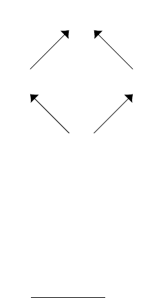
(on the right):
µ
1
= µ
F
= (,f
3
,
|
w
1
,f
2
,
|
w
2
,f
1
,
|
w
3
,f
4
,
|
w
4
)
µ
2
= (f
3
, ,f
1
, ,f
2
, ,f
4
)
µ
3
= (f
4
, ,f
2
, ,f
1
, ,f
3
)
µ
4
= µ
W
= (f
4
, ,f
1
, ,f
2
, ,f
3
)
µ
4
µ
3
µ
2
µ
1
On the left, we use a compact notation for matchings by specifying partners of workers w
1
,
w
2
, and so forth. In the lattice on the right, workers prefer “higher” stable matchings with
µ
4
= µ
W
being the worker-optimal stable matching.
Just for illustration, consider the following unstable matching (underlined in the matrix
above)
λ = (w
1
, f
1
, f
2
, f
3
)
obtained from the worker-optimal stable matching µ
W
by unmatching worker w
1
with his
stable partner, firm f
4
. Since there is a path of length 1 from λ back to µ
W
, we call λ almost
(worker-optimal) stable.
Then, there is a path of length 5 from this almost worker-optimal stable matching to the
firm-optimal stable matching µ
F
(in bold):
λ = λ
0
−−−−→
(f
3
,w
1
)
λ
1
−−−−→
(f
1
,w
4
)
λ
2
−−−−→
(f
2
,w
2
)
λ
3
−−−−→
(f
4
,w
4
)
λ
4
−−−−→
(f
1
,w
3
)
λ
5
= µ
F
,
where under the “transition” arrows above, we specify blocking pairs chosen at each step.
More importantly, in this example, there is a path from any unstable matching to any
stable one. This will follow from our analysis in Section 3. △
8
Example 2. Now, consider another example with four firms and four workers:
1, 1 2, 2 3, 4 4, 2
4, 3 2, 3 1, 2 3, 1
2, 2 1, 4 4, 3 3, 4
3, 4 4, 1 2, 1 1, 3
.
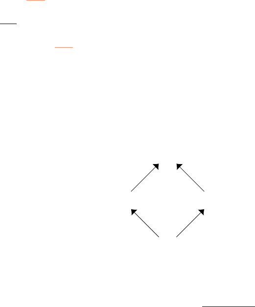
Even though the agents’ preferences are slightly different, the structure of stable match-
ings is similar:
µ
1
= µ
F
= (f
2
, f
4
, f
3
, f
1
)
µ
2
= (f
2
, f
4
, f
1
, f
3
)
µ
3
= (f
4
, f
2
, f
3
, f
1
)
µ
4
= µ
W
= (f
4
, f
2
, f
1
, f
3
)
µ
4
µ
3
µ
2
µ
1
In contrast to the previous example, for some unstable matchings, we cannot attain all
stable ones. In particular, the following almost worker-optimal stable matching (underlined
in the ordinal payoff matrix)
λ = (w
1
, f
2
, f
1
, f
3
)
can only reach stable matchings µ
2
and µ
W
, but not, say, firm-optimal stable µ
F
.
So what is driving this difference between two examples? Consider the submarket formed
by firms
¯
F = {f
1
, f
3
} and workers
¯
W = {w
3
, w
4
} (in orange) and focus on the following
matching for this submarket (in bold)
¯µ = (,f
1
,
|
w
3
,f
3
,
|
w
4
),
according to which worker w
3
is matched with firm f
1
and w
4
is matched with firm f
3
.
This matching ¯µ has two features. First, it is stable for the considered submarket. Second,
9
every agent inside the submarket prefers her stable partner under ¯µ to every agent outside
the submarket. In such case, we say that firms
¯
F and workers
¯
W form a fragment that is
induced by matching ¯µ.
Together these two features imply that any matching in the original market agreeing with
¯µ cannot break any partnership implied by ¯µ, and thus cannot attain any stable matching
disagreeing with ¯µ. When not all stable matchings agree on a fragment (as in this example),
we call it non-trivial.
Going back to our underlined matching λ, it agrees with inducing ¯µ and therefore cannot
attain stable matchings µ
F
and µ
3
that instead disagree. That is, λ can potentially reach
only stable µ
2
and µ
W
. In fact, it is easy to check that it can reach both.
In Section 3.3, we show that the absence of non-trivial fragments is not only necessary,
but also sufficient to have a path from any unstable matching to any stable one.
Note however that even when we have fragments, usually only a small proportion of initial
matchings can be trapped by them. In this particular example, any unstable matching that
disagrees with ¯µ can actually attain any stable matching. Furthermore, those that agree can
still attain both µ
2
and µ
W
. △
3.2. Fragments: Definitions and Properties. In this subsection, we formally define
fragments and discuss their properties.
Suppose
¯
F ⊊ F and
¯
W ⊊ W are such that |
¯
F | = |
¯
W | = k ∈ [n − 1] and let
¯
M be the
market induced by the original market M when restricted to
¯
F ∪
¯
W . Firms
¯
F and workers
¯
W
constitute a fragment (of size k) in M if there exists a stable matching ¯µ :
¯
F ∪
¯
W →
¯
F ∪
¯
W
for
¯
M such that (i) for any
¯
f ∈
¯
F and w /∈
¯
W , ¯µ(
¯
f) ≻
¯
f
w, and (ii) for any ¯w ∈
¯
W and
f /∈ F , ¯µ( ¯w) ≻
¯w
f. In this case, we say that ¯µ induces fragment (
¯
F ,
¯
W ).
There are several properties of fragments. First, we might have multiple fragments
(nested, overlapping, or disjoint). Second, a fragment might be induced by multiple match-
ings ¯µ, see Example 5 in Appendix A. Third, for any given inducing matching, we can find
10
a stable matching in the original market that agrees with the inducing one over its corre-
sponding fragment (Lemma 2 in Appendix A). The converse is not true; that is, a stable
matching in the original market might disagree with all matchings inducing a fragment (e.g.,
stable µ
F
and µ
3
disagree with the unique inducing matching ¯µ in Example 2). Finally, and
more importantly, fragments have the following defining property.
Lemma 1. Suppose there is a fragment (
¯
F ,
¯
W ) in the original market. Then, for any stable
matching µ in the original market, µ(
¯
F ) =
¯
W .
This lemma says that any stable matching in the original market must match agents
inside a fragment within the fragment. It works for all stable matchings, including those
that disagree with each other or with all inducing matchings on how they match agents
inside the fragment. In particular, it holds for stable µ
F
and µ
3
disagreeing with inducing ¯µ
in Example 2. That is why the word “fragment” seems to be an appropriate name.
Intuitively, consider fragment (
¯
F ,
¯
W ) (of size k ∈ [n−1]) that, up to relabeling, is induced
by ¯µ(f
i
) = w
i
, for any i ∈ [k]. Assume, for sake of contradiction, that µ(
¯
F ) ̸=
¯
W for some
stable µ in the original market. Then, up to relabeling, µ(w
1
) /∈
¯
F , and therefore worker
w
1
prefers his “inside” partner under ¯µ, firm f
1
∈
¯
F , to his “outside” partner under µ, firm
µ(w
1
) /∈
¯
F . By stability of µ, firm f
1
must in turn prefer her partner under µ over her
“inside” partner under ¯µ, worker w
1
. By definition of inducing ¯µ, f
1
’s partner under µ must
be also inside the fragment. Up to relabeling, let µ(f
1
) = w
2
∈
¯
W .
Next, by stability of inducing ¯µ, worker w
2
must prefer his partner under ¯µ, firm f
2
∈
¯
F ,
to his partner under µ, firm f
1
∈
¯
F . As above, by using first stability of µ and then
definition of inducing ¯µ, f
2
’s partner under µ must be inside the fragment. Up to relabeling,
let µ(f
2
) = w
3
∈
¯
W .
By proceeding recursively, all firms inside the fragment must be matched to different
workers inside the fragment under given stable µ. This contradicts our assumption µ(
¯
F ) ̸=
¯
W , and thus proves the lemma.
A fragment is called trivial if all stable matchings in the original market agree on how
11
they match agents within the fragment. Equivalently, triviality means that the corresponding
fragment has a unique inducing matching that all stable matchings in the original market
agree with over the fragment. Thus, it is stronger than the Lemma 1’s conclusion.
For instance, a pair (f
i
, w
j
) of mutually most preferred agents constitutes a trivial frag-
ment of size 1. Such pair is called a top-top match. In addition, a sequence of k < n such
pairs—where each new top-top pair in the sequence is obtained from the submarket after
removing all previous top-top pairs from the original market—forms a trivial fragment of size
k. But trivial fragments are not limited to such sequences, see Example 6 in Appendix A.
Returning to Example 2, the corresponding market has the unique fragment (
¯
F ,
¯
W )
that is non-trivial. Indeed, even though it has the unique inducing matching ¯µ, only stable
matchings µ
2
and µ
W
agree with ¯µ on the fragment, but not µ
F
and µ
3
. In Section 3.3, we
show that the presence of non-trivial fragments is closely related to non-reachability.
3.3. Characterization Result. Before stating the first theorem, we introduce some defi-
nitions and notation.
A matching is called almost stable if it has a path of length 1 to a stable matching. In
fact, for balanced markets, a matching µ
−f
is almost stable if it is obtained from a stable
matching µ by unmatching firm f ∈ F with her stable partner µ(f ). By definition, any
almost stable matching is unstable. Note however that almost stable matchings constitute
only a tiny fraction of all unstable matchings.
To make our result stronger, we place an additional restriction on paths. As motivation,
consider again Example 1. We obtained the path from almost worker-optimal stable λ = λ
0
to firm-optimal stable µ
F
= λ
5
. In that path, to get λ
1
in the first step, we satisfy the
blocking pair (f
3
, w
1
) that is the best for firm f
3
among all her blocking pairs under λ
0
;
indeed, (f
3
, w
1
) is the only blocking pair for f
3
. Next, to attain λ
2
in the second step, we
satisfy the f
1
’s best blocking pair, (f
1
, w
4
), among all her blocking pairs under current λ
1
.
12
In fact, the considered path
λ = λ
0
f
3
-best
−−−−→
(f
3
,w
1
)
λ
1
f
1
-best
−−−−→
(f
1
,w
4
)
λ
2
w
2
-best
−−−−→
(f
2
,w
2
)
λ
3
f
4
-best
−−−−→
(f
4
,w
4
)
λ
4
f
1
-best
−−−−→
(f
1
,w
3
)
λ
5
= µ
F
can be rationalized by the sequence (f
3
, f
1
, w
2
, f
4
, f
1
) of agents from both sides sequentially
choosing their best blocking pairs among all blocking pairs available in their turn.
For the theorem below, restrict attention to paths that can be rationalized in the sense
defined in the previous paragraph.
Theorem 1. The following three statements are equivalent:
(i) any unstable matching can attain any stable matching;
(ii) any almost stable matching can attain any stable matching;
(iii) there are no non-trivial fragments.
This result suggests fragility of stable matchings. Indeed, consider stable µ and perturb it
arbitrarily to obtain unstable λ; perhaps, even “minimally” to get an almost stable matching
that is just one blocking pair away from µ. Then, if there are multiple stable matchings, λ
might diverge to any other—possibly “distant”—stable matching.
In Section 4.2, we show this fragility is not just an artefact of constructed deterministic
paths, but can also emerge when at each step, a blocking pair to be satisfied is chosen
randomly (Roth and Vande Vate, 1990).
Here, we provide a brief sketch of the proof, full details of which are relegated to Ap-
pendix C. It suffices to prove (i) ⇒ (iii) ⇒ (ii) ⇒ (i). In order to show (i) ⇒ (iii), we prove
¬(iii) ⇒ ¬(i). Note that any unstable matching λ that agree with an inducing matching over
its corresponding non-trivial fragment can only attain those stable matchings that also agree.
By non-triviality, there are stable matchings that disagree, and thus cannot be attained by
λ, as in Example 2.
13

Next, to prove (ii) ⇒ (i), consider any unstable λ. It is enough to show there is a path to
a stable matching µ. Indeed, in that case, there must be also a path to almost stable µ
−f
,
for some f ∈ F , from which we then can attain any stable matching by (ii), as required.
One technical issue is that, due to our restriction on paths, we cannot rely on the Roth and
Vande Vate (1990)’s theorem when constructing paths to stability. In our proof, we instead
employ the recent extension by Ackermann et al. (2011) who showed existence of stable paths
compatible with our restriction.
7
Finally and most importantly, regarding (iii) ⇒ (ii), why can we attain all stable match-
ings in markets with no non-trivial fragments? The high-level intuition is that the absence of
non-trivial fragments effectively allows to emulate all operations in the McVitie and Wilson
(1971)’s algorithm designed to find all stable matchings.
As a small digression, McVitie and Wilson (1971) adapted the firm-proposing DA by
introducing a new operation called breakmarriage to determine the set of all stable matchings
starting from firm-optimal µ
F
. For any stable µ and any paired firm f with µ(f) = w ∈ W ,
the operation breakmarriage(µ, f) is roughly defined as follows (see full details and relevant
results in Appendix B). It (a) “breaks” the (f, w)-partnership making f and w free, (b) and
restarts the previously terminated DA by forcing firm f to propose to the worker following
w in her list, thus initiating a new sequence of proposals, rejections and acceptances as given
by the restarted DA (Gusfield, 1987). It turns out that any stable µ ̸= µ
F
can be obtained
from µ
F
by successive applications of the breakmarriage operation.
Returning to the proof sketch, we use induction on the size n = |F | = |W | of markets
with no non-trivial fragments. The result holds for n = 1. Assume it holds for all such
markets of at most size (n − 1). Consider any such market of size n with arbitrary almost
stable λ corresponding to stable µ.
By using our induction hypothesis and the definition of non-trivial fragments, we first
show that λ can attain either any stable matching, so the result follows immediately, or any
7
In fact, Ackermann et al. (2011) proved existence of stable paths rationalized by sequences of agents
from one side (i.e., only firms or only workers) successively selecting their best blocking pairs.
14

almost stable matching µ
−f
corresponding to µ. The latter case implies we can emulate part
(a) of the breakmarriage operation for stable µ. Indeed, any almost stable µ
−f
is obtained
from µ by “breaking” the (f, µ(f))-partnership.
Moreover, we show how to emulate part (b) of the breakmarriage operation. This nat-
urally follows from the DA procedure (Lemma 3 in Appendix B) and holds irrespective of
whether we have non-trivial fragments or not.
Therefore, for given stable µ, we can emulate any breakmarriage(µ, f) operation, f ∈ F ,
and reach some other stable matchings, different from µ.
For each newly attained stable ν ̸= µ, we can also reach its almost stable ν
−f
′
, for some
f
′
∈ F , and repeat the same analysis as for λ, but now for ν
−f
′
. Namely, we can reach either
any stable matching, as desired, or emulate any breakmarriage(ν, f) operation, f ∈ F .
By iteratively employing this procedure, we can attain any stable matching from initial
almost stable λ corresponding to stable µ. Indeed, we can effectively emulate all operations
both in the original McVitie and Wilson (1971)’s algorithm with firms proposing, described
above, and in its symmetric version with workers proposing. By simultaneously using both
versions, we can obtain any stable matching starting from any given stable matching, in-
cluding µ, i.e. not necessarily from firm- or worker-optimal ones (see details in the proof).
To conclude, we argue that the absence of non-trivial fragments is a mild condition.
Indeed, Figure 1 suggests non-trivial fragments are rare for balanced markets (of size n =
|F | = |W |) with uniformly random preferences.
8
Even though the frequency of markets with
non-trivial fragments is increasing for sizes up to n = 7, it is never above 20% and eventually
decreasing. We conjecture it converges to zero as n goes to infinity. Therefore, we expect
Theorem 1 to hold generically in this setting.
At the same time, uniformly random balanced markets have many stable matchings with
significantly different welfare properties. Formally, Pittel (1989) proved that the expected
8
Figure 1 relies on simulated markets, the number of which varies from 500 (for larger market sizes n) to
20,000 (for smaller n).
15
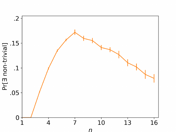
Figure 1: Frequency of uniformly random balanced markets of size n with non-trivial
fragments
number of stable matchings is asymptotic to e
−1
n ln n. Moreover, the firms’ average ranks of
their assigned workers under firm-optimal (n/ ln n) and worker-optimal (ln n) stable match-
ings are significantly different. Symmetric results hold for workers.
Each of those numerous stable matchings, when perturbed arbitrarily—perhaps, even
“minimally”—might diverge to any other stable matching, possibly with completely different
welfare properties. We will discuss it further in Section 4.2.
4. Quantifying Fragility of Stable Matchings
In this section, we examine fragility of stable matchings with respect to “small” perturbations
by assuming that at each step of the rematching process, a blocking pair to be satisfied is
chosen uniformly at random.
We analyze two fragility measures. For either measure, we pick a stable matching and
perturb it a little bit to obtain a “close” unstable matching, possibly an almost stable one.
Motivated by Theorem 1, we first consider markets with multiple stable matchings and
quantify fragility by using return probabilities. For such markets, an arbitrarily—perhaps,
“minimally”—perturbed stable matching may be more likely to diverge to some other po-
16

tentially “distant” stable ones. We employ simulations and examples to demonstrate that
(i) some stable matchings are more robust than others; (ii) extremal stable matchings, usually
targeted by centralized matching mechanisms, may be most fragile; (iii) all stable matchings
might be fragile.
Since for markets with a unique stable matching return probabilities have no bite, we use
an expected path length to regain stability as another fragility measure. We prove that any
such market can be extended, in a “small” way, so that in the extended market, after almost
any perturbation including “small” ones, the rematching process needs at least exponentially
many steps to restore stability; see Theorem 2.
4.1. Type 1: Expected Path Length. We begin our analysis by considering markets
with unique stable matchings. For an arbitrary such market, any unstable matching—
including all perturbations of the corresponding unique stable matching—converges with
probability one back to that stable matching. In other words, any unique stable matching
is not fragile in the sense of Theorem 1.
Nonetheless, even a unique stable matching can be fragile to “small” perturbations, but
in a different sense. To be more precise, it might require a long time, i.e. many steps, in
order to restore stability.
In what follows, we show that any market can be “slightly” extended in a way that pre-
serves uniqueness and preferences of original agents over each other, so that in the extended
market almost any, possibly very “small,” perturbation of the corresponding unique stable
matching with high probability leads to at least exponentially long paths to stability.
Our analysis is partially motivated by Ackermann et al. (2011), the first paper provided an
exponential lower bound for the convergence time, but has several important differences. To
provide this bound, they considered just one market instance with many stable matchings and
focused on some, not all, initial matchings. In contrast, we analyze arbitrary markets having
unique stable matchings and examine their robustness with respect to “small” perturbations.
9
9
Even though we focus on markets with unique stable matchings, we believe similar techniques can be
17

In addition, Ackermann et al. (2011) identified a class of markets with no preference cycles,
in which irrespective of a starting matching the convergence time is polynomial.
10
Since any
market in this class has a unique stable matching, our analysis suggests that when “slightly”
extended, the convergence time becomes at least exponential for almost any perturbation.
Formally, given δ ≥ 0, a δ-augmented market of the original market of size n is a new
market of size at most (1+δ)n obtained from the original one by adding at most δ-proportion
of new agents on both sides, so that (i) both original and augmented markets coincide when
restricted to the original agents; (ii) the augmented market has a unique stable matching;
(iii) all original agents have identical stable partners in both markets.
Also, given ϵ > 0, we say a matching is ϵ-unstable if at least ϵ-fraction of firms, and thus
workers, are not matched with their (unique) stable partners.
Theorem 2. Consider any sequence of markets of size n ∈ N and any δ, ϵ > 0. Then,
there is a sequence of corresponding δ-augmented markets so that any sequence of ϵ-unstable
matchings with probability 1 − 2
−Ω(n)
needs 2
Ω(n)
steps to regain stability.
11
To provide an intuition behind our construction, we sketch the main proof steps. First,
we prove the same convergence result for a sequence of non-augmented markets of size n ∈ N,
such that for some fixed η > 0, every market in the sequence satisfies the following condition:
any agent on one side except one is preferred by at least η-proportion of agents from the
other side to their stable partners (see Proposition 1 in Appendix C). Up to several technical
differences, the proof idea is similar to Ackermann et al. (2011). Intuitively, when we are
close to stability, there are much more “destabilizing” blocking pairs moving us away from
stability than “stabilizing” blocking pairs leading us towards stability. Indeed, when many
agents are already matched with their stable partners, any unmatched firm (or worker)—
except the one excluded in the condition—makes a large proportion of workers (respectively,
used to extend our result to arbitrary markets.
10
In fact, this result can be easily generalized to a larger class of markets, also with unique stable matchings,
satisfying the so-called sequential preference condition (Eeckhout, 2000).
11
We write f (n) = Ω(g(n)) if g(n) = O(f(n)).
18

firms) want to break their stable partnerships. By using this observation, we connect our
rematching process to a biased random walk that is more likely to move away from stability,
and thus requires a long time to eventually obtain it.
As a side note, there is no market with a unique stable matching such that any agent
on one side, without any exceptions, is preferred by some agents from the other side to
their stable partners.
12
That is why in the condition above, we require one exception for
workers and one exception for firms. Even though it complicates the analysis, compared to
Ackermann et al. (2011), analogous techniques can be used to prove Proposition 1.
Next, we show there are indeed sequences of non-augmented markets that satisfy the
conditions of Proposition 1 and construct one such sequence. In fact, this class is quite
broad and might include “almost” fully assortative markets, in which all agents on one side
agree on how they rank the vast majority of all agents from the other side.
Finally, we employ the constructed sequence to extend arbitrary markets and prove the
main result. Consider any sequence of markets of size n ∈ N and any δ > 0. Then, for any
market (of size n) in the sequence, we add new agents with preferences over each other that
replicate the constructed market of size ⌊δn⌋. We assume that both original and new firms
(or workers) prefer any original worker (respectively, firm) to any new one. The constructed
market is indeed δ-augmented and satisfies the similar conditions as in Proposition 1, despite
being extended, so the result follows.
To conclude, simulations (available upon request) suggest similar fragility results emerge
for uniformly random markets, both with no restrictions and with unique stable matchings.
In particular, for markets of size n = 10 with no restrictions, an almost stable matching—
that is just one blocking pair away from stability—on average requires around 90 periods
to converge to a stable matching, not necessarily the original one. Furthermore, the re-
equilibration process usually involves many agents being unmatched and rematched for a
substantial number of periods.
12
This follows from Lemma 7 in Balinski and Ratier (1997).
19

4.2. Type 2: Return Probability. Now, focus on markets with multiple stable matchings
and, as before, assume that at each step, a blocking pair to be satisfied is chosen uniformly
at random (Roth and Vande Vate, 1990).
For this random setting, Theorem 1 implies that for markets with no non-trivial frag-
ments, any stable matching, when perturbed arbitrarily, might attain any stable matching
with positive probability.
13
In particular, there is a positive probability to diverge from the
original stable matching to some other, possibly “distant,” stable ones.
In fact, even when we have non-trivial fragments, the same fragility issue might emerge.
As discussed in Example 2, usually only a tiny fraction of initial matchings, and thus per-
turbations of stable matchings, might be trapped by fragments and unable to attain all
stable matchings. Moreover, even those that are trapped might still potentially reach some
non-singleton subset of stable matchings.
In what follows, we use the insights above as well as our uniformly random setting to
measure and compare fragility of different stable matchings. As an illustration, consider the
following simple market
2, 1 1, 2
1, 2 2, 1
with two stable matchings, µ
F
= (f
1
, f
2
) and µ
W
= (f
2
, f
1
). Up to permutations, it is the
only balanced market of size n = 2 with multiple stable matchings.
Next, perturb “minimally” firm-optimal stable µ = µ
F
to obtain almost stable λ =
µ
−f
2
= (f
1
, w
2
) that is just one blocking pair away from µ
F
(the same analysis would hold
for λ = µ
−f
1
). What is the probability for almost stable λ to return back to stable µ
F
?
14
Let r denote the corresponding return probability.
Notice λ has two blocking pairs, (f
2
, w
1
) and (f
2
, w
2
). Both are equally likely to be
13
Both multiplicity of stable matchings and lack of non-trivial fragments are likely to hold in larger balanced
markets, see our discussion in Section 3.3.
14
The perturbations leading to almost stable matchings are “minimal” in the sense that in order to return
back to µ, any other unstable matching—corresponding to any other perturbation—must attain some of µ’s
almost stable matchings.
20

satisfied. With the probability of 1/2, we satisfy (f
2
, w
2
), and converge with probability
one back to µ
F
. With the remaining probability of 1/2, we instead satisfy (f
2
, w
1
) and
attain almost stable ν
−f
1
= (f
2
, w
2
), now corresponding to worker-optimal stable ν = µ
W
.
By symmetry, ν
−f
1
returns back to µ
W
with probability r, and thus diverges to µ
F
with
probability (1 − r). Therefore,
r = 1/2 × 1 + 1/2 × (1 − r) =⇒ r = 2/3.
In addition, we will be interested in the return probability conditional on not regaining
stability in the first step. For this example, the conditional return probability is
r
c
= 1 − r = 1/3.
Since the example is symmetric, any other almost stable matching has the same measures r
and r
c
, as calculated above.
Motivated by this example, we calculate (conditional) return probabilities for randomly
chosen almost stable matchings in random markets. To be more precise, we sample uniformly
random balanced markets with multiple stable matchings of different sizes n ∈ [10], with
1000 draws per each n. For each such market, we pick three stable matchings: firm-optimal
µ
F
, worker-optimal µ
W
, and stable µ
R
chosen uniformly at random (might coincide with
either µ
F
or µ
W
). For each such stable µ
T
, T ∈ {F, W, R}, we choose its one almost stable
matching λ
T
, also uniformly at random. Next, for each market and each almost stable
matching λ
T
, we calculate both its corresponding return probability and conditional return
probability (if applicable).
15
Finally, for each market size n and each type T of almost stable
matchings, we take expectation over respective (conditional) return probabilities.
Figure 2 shows expected (conditional) return probabilities. Even though the expected
15
For n ≤ 5, we use the Markov structure of the problem with states being all matchings to calculate exact
return probabilities. For n > 6, it becomes computationally infeasible and we instead use simulations, based
on 500 simulated paths.
21
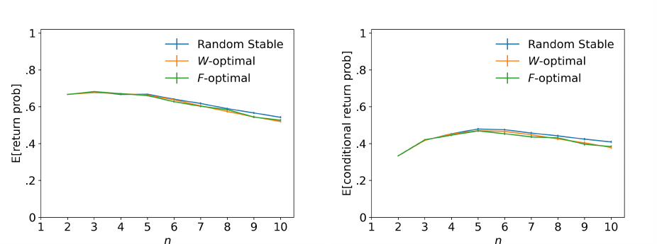
return probability (on the left) is slightly increasing for small n, it is eventually decreasing.
In particular, for all stable matchings, it is around 50% for balanced markets of size n = 10.
In other words, for such markets, when perturbed “minimally,” stable matchings return back
only with probability 50%. Furthermore, random stable matchings seem to be more robust
than extremal ones for larger sizes n. In turn, extremal stable matchings are equally robust,
since markets are balanced. As concern conditional probabilities (on the right), they are
naturally smaller, but exhibit similar patterns.
(a) Return probability (b) Conditional return probability
Figure 2: Expected return probabilities and conditional return probabilities for uniformly
random markets of size n with multiple stable matchings
Figure 3 depicts distributions of (conditional) return probabilities for larger market sizes
n = 8, 9, 10. Stable matchings have different return probabilities, most of which are smaller
than one. In particular, some stable matchings are more robust than others. Moreover, as
n increases, these distributions flatten implying stable matchings become more fragile.
So far, we showed that when perturbed a little bit, a stable matching might diverge to
some other stable matchings with substantial probability. Can it potentially diverge to some
“distant” stable matchings with different welfare properties?
In fact, similar fragility patterns hold even for markets with two completely different
stable matchings, in which each agent has two different stable partners. In Example 3
below, we present one such market and argue that it has only one robust stable matching.
22
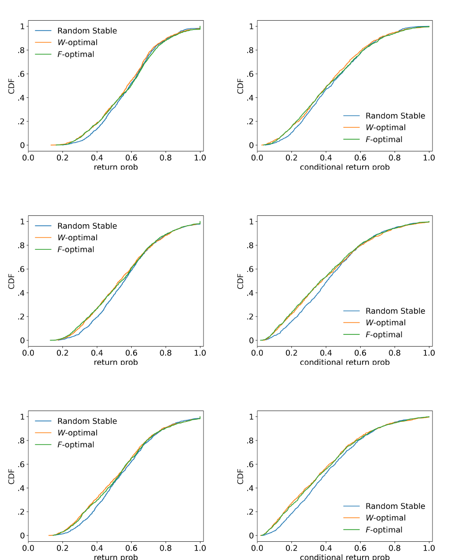
(a) n = 8
(b) n = 9
(c) n = 10
Figure 3: Distribution of return probabilities (Left) and conditional return probabilities
(Right) for uniformly random markets of size n with multiple stable matchings
23

Example 3. Consider the following market with six firms and six workers:
6, 2 4, 5 3, 1 2, 6 5, 2 1, 6
3, 6 5, 1 2, 4 6, 3 4, 6 1, 5
5, 5 3, 3 6, 2 4, 1 2, 4 1, 3
1, 1 4, 2 5, 3 6, 4 3, 1 2, 2
3, 4 2, 6 1, 6 5, 2 6, 3 4, 4
1, 3 2, 4 3, 5 5, 5 4, 5 6, 1
.
There are two stable matchings:
µ
F
= (f
1
, f
2
, f
3
, f
4
, f
5
, f
6
) and µ
W
= (f
3
, f
1
, f
4
, f
6
, f
2
, f
5
),
so that each agent has two different stable partners.
By using the Markov structure of the problem with states being matchings, we calculate
both return probabilities
stable \ unmatch w
1
w
2
w
3
w
4
w
5
w
6
µ
F
= (f
1
, f
2
, f
3
, f
4
, f
5
, f
6
) 0.3108 0.2657 0.2706 0.2769 0.2689 0.2362
µ
W
= (f
3
, f
1
, f
4
, f
6
, f
2
, f
5
) 0.9883 0.9810 0.9886 0.9825 0.9801 0.9819
and conditional return probabilities
stable \ unmatch w
1
w
2
w
3
w
4
w
5
w
6
µ
F
= (f
1
, f
2
, f
3
, f
4
, f
5
, f
6
) 0.0811 0.0821 0.0883 0.0962 0.0861 0.0834
µ
W
= (f
3
, f
1
, f
4
, f
6
, f
2
, f
5
) 0.9766 0.9747 0.9772 0.9781 0.9761 0.9758
for all almost stable matchings. Namely, for each stable µ ∈ {µ
F
, µ
W
} and every i ∈ [6],
we obtain almost stable µ
−w
i
from µ by unmatching w
i
—corresponding to column names
above—with his stable partner µ(w
i
) and compute its corresponding return probabilities.
24

These results imply that firm-optimal stable µ
F
is fragile with respect to arbitrary per-
turbations. Indeed, each of its almost stable matchings is more likely to diverge to worker-
optimal stable µ
W
. In fact, irrespective of how close we start to µ
F
, in order to return back,
one needs to attain one of its almost stable matchings, and thus is more likely to attain µ
W
instead. In that sense, almost stable matchings corresponding to “minimal” perturbations
provide lower bounds on fragility; see footnote 14.
In contrast, worker-optimal stable µ
W
seems robust. Even though, when perturbed a
little bit, it can still diverge to µ
F
, this is very unlikely. Interestingly, robust stable µ
W
is
more egalitarian than fragile stable µ
F
.
16
△
To conclude, we note there are some markets with no robust stable matchings, as illus-
trated in Example 4.
Example 4. Consider the following market with six firms and six workers:
6, 1 5, 2 4, 3 3, 4 2, 5 1, 6
1, 6 6, 1 5, 2 4, 3 3, 4 2, 5
2, 5 1, 6 6, 1 5, 2 4, 3 3, 4
3, 4 2, 5 1, 6 6, 1 5, 2 4, 3
4, 3 3, 4 2, 5 1, 6 6, 1 5, 2
5, 2 4, 3 3, 4 2, 5 1, 6 6, 1
.
It has six stable matchings
µ
1
= µ
F
= (f
1
, f
2
, f
3
, f
4
, f
5
, f
6
)
µ
2
= (f
6
, f
1
, f
2
, f
3
, f
4
, f
5
)
µ
3
= (f
5
, f
6
, f
1
, f
2
, f
3
, f
4
)
µ
4
= (f
4
, f
5
, f
6
, f
1
, f
2
, f
3
)
µ
5
= (f
3
, f
4
, f
5
, f
6
, f
1
, f
2
)
µ
6
= µ
W
= (f
2
, f
3
, f
4
, f
5
, f
6
, f
1
)
16
In our simulations, more egalitarian stable matchings seem to be more robust on average (results available
upon request). Nevertheless, in particular markets, the most egalitarian stable matching is not necessarily
the most robust one, see Boudreau (2011) for a related observation.
25
corresponding to six “diagonals” in the matrix.
As before, we compute exact values for return probabilities
stable \ unmatch w
i
, any i
µ
F
= (f
1
, f
2
, f
3
, f
4
, f
5
, f
6
) 0.2010
µ
2
= (f
6
, f
1
, f
2
, f
3
, f
4
, f
5
) 0.3165
µ
3
= (f
5
, f
6
, f
1
, f
2
, f
3
, f
4
) 0.5035
µ
4
= (f
4
, f
5
, f
6
, f
1
, f
2
, f
3
) 0.5035
µ
5
= (f
3
, f
4
, f
5
, f
6
, f
1
, f
2
) 0.3165
µ
W
= (f
2
, f
3
, f
4
, f
5
, f
6
, f
1
) 0.2010
and conditional return probabilities
stable \ unmatch w
i
, any i
µ
F
= (f
1
, f
2
, f
3
, f
4
, f
5
, f
6
) 0.0412
µ
2
= (f
6
, f
1
, f
2
, f
3
, f
4
, f
5
) 0.1798
µ
3
= (f
5
, f
6
, f
1
, f
2
, f
3
, f
4
) 0.4042
µ
4
= (f
4
, f
5
, f
6
, f
1
, f
2
, f
3
) 0.4042
µ
5
= (f
3
, f
4
, f
5
, f
6
, f
1
, f
2
) 0.1798
µ
W
= (f
2
, f
3
, f
4
, f
5
, f
6
, f
1
) 0.0412
for each almost stable matching. By symmetry, it suffices to calculate only three return
probabilities and three conditional return probabilities.
Note first that all stable matchings seem fragile. Furthermore, extremal stable matchings
are most fragile, similar to Figures 2 and 3. Finally, as in Example 4, more egalitarian stable
matchings are less fragile, see footnote 16. △
26

Appendix A. Properties of Fragments
In this appendix, we provide more details behind the properties of fragments and induced
matchings stated in Section 3.2
Example 5 shows that a fragment might be induced by multiple matchings ¯µ.
Example 5. Consider the following market with four firms and four workers:
U =
1, 4 3, 4 2, 2 4, 3
3, 3 2, 1 4, 3 1, 1
4, 1 3, 2 1, 4 2, 2
1, 2 4, 3 2, 1 3, 4
.
Firms
¯
F = {f
1
, f
4
} and workers
¯
W = {w
2
, w
4
} form a fragment that can be induced by
either
¯µ
1
= (,f
1
,
|
w
2
,f
4
,
|
w
4
) or ¯µ
2
= (,f
4
,
|
w
2
,f
1
,
|
w
4
). △
Next, we show that for any given inducing matching, we can find a stable matching in
the original market that agrees with the inducing one over its corresponding fragment.
Lemma 2. Consider any ¯µ that induces fragment (
¯
F ,
¯
W ). Then, there exists a stable match-
ing µ for the original market that agrees with ¯µ when restricted to
¯
F ∪
¯
W .
17
Proof. The submarket obtained from the original market by removing the given fragment
has a stable matching. Any such stable matching combined with the inducing matching
constitutes a stable matching in the original market, as desired.
As we discuss in the main text, the converse does not hold. Namely, a stable matching
in the original market might disagree with all matchings inducing a fragment. For instance,
stable matchings µ
F
and µ
3
disagree with the unique inducing matching ¯µ in Example 2.
17
This lemma implies that only “projections” of stable matchings in the original market might potentially
induce fragments. Thus, given all stable matchings, one can effectively find all fragments.
27
The final example in this appendix demonstrates that a trivial fragment does not necessar-
ily correspond to a sequence of top-top match pairs (see Section 3.2 for relevant definitions).
Example 6. Consider the following market with four firms and four workers:
2, 4 1, 4 3, 2 4, 3
3, 3 2, 1 4, 3 1, 1
4, 1 3, 2 1, 4 2, 2
2, 2 4, 3 3, 1 1, 4
.
There are two stable matchings:
µ
F
= (f
3
, f
4
, f
2
, f
1
) and µ
W
= (f
2
, f
4
, f
3
, f
1
).
Since both stable matchings agree with
¯µ = (,f
4
,
|
w
2
,f
1
,
|
w
4
)
inducing fragment (
¯
F ,
¯
W ) = ({f
1
, f
4
}, {w
2
, w
4
}), the considered fragment is trivial. However,
there are no top-top matches in this market. △
Appendix B. McVitie and Wilson (1971)’s Algorithm
Gale and Shapley (1962) showed that the set of stable matchings is non-empty for any
matching market. In doing so, they introduced the deferred acceptance algorithm (DA)
described below:
Step 1. Each firm proposes to her favorite (acceptable) worker (if any). Each worker
who receives more than one offer, tentatively holds on to his favorite (acceptable) one
(if any), and rejects all others.
28

Step k. Each firm who was rejected in step (k − 1) makes an offer to her favorite
(acceptable) worker who has not rejected her yet (if any). Each worker holds his most
preferred acceptable offer to date (if any), and rejects all others.
Stop. When no further proposals are made, match each firm to the worker (if any)
whose proposal he is holding.
The description above corresponds to the firm-proposing DA. Gale and Shapley (1962)
proved that its output is the firm-optimal stable matching µ
F
: each firm weakly prefers
her assigned partner under this matching to the partner she would get in any other stable
matching. The worker-proposing DA defined in a similar way produces the worker-optimal
stable matching µ
W
. In fact, firms and workers have opposing interests with regard to stable
matchings: if firms prefer one stable matching over another, workers hold the opposite
opinion (Knuth, 1976).
18
In particular, the firm-optimal (worker-optimal) stable matching
is also worker-pessimal (firm-pessimal). Furthermore, the set of unmatched agents is the
same across all stable matchings (according to the so-called “rural hospital theorem” proved
by McVitie and Wilson, 1970).
McVitie and Wilson (1971) developed an alternative sequential version of the firm-
proposing DA, in which proposals by firms to workers are made one at a time (and in
an arbitrary order), but not simultaneously as in the Gale and Shapley (1962)’s algorithm.
However, both versions result in the same set of proposals and in the same firm-optimal
stable matching µ
F
.
Importantly, McVitie and Wilson (1971) also adapted the firm-proposing DA by using
an operation called breakmarriage to determine the set of all stable matchings starting from
the firm-optimal one. In the paper, they considered a balanced market, i.e. n = m, with
all agents being acceptable. In what follows, we provide extended results that allow for a
market imbalance and unacceptable agents.
For any stable matching µ and any paired firm f with µ(f ) = w ∈ W , the operation
18
In fact, the set of stable matchings forms a distributive lattice (proved by Conway, see Knuth, 1976).
29

breakmarriage(µ, f) is defined as follows. It “breaks” the (f, w)-partnership making firm
f free and worker w “semi-free” in the sense that he will only accept a proposal from a
firm he prefers to f (Gusfield, 1987). This forces firm f to propose to the worker following
w in her list, thus initiating a sequence of further proposals, rejections, and (tentative)
acceptances according to the restarted firm-proposing DA. As there is at most one free firm
that has not yet run out of her acceptable alternatives at any time,
19
the corresponding
process is deterministic and terminates when (i) worker w receives a proposal from a firm
he prefers to his current partner f, or (ii) some previously matched firm runs out of her
acceptable alternatives, or (iii) some previously unmatched worker receives a proposal from
an acceptable firm. In the first case, the process is called successful and leads to a new stable
matching µ
′
̸= µ (Theorem 3 in McVitie and Wilson, 1971, also stated as a lemma below).
Lemma (McVitie and Wilson, 1971). Consider any stable matching µ and any paired
firm f with µ(f) = w ∈ W . If breakmarriage(µ, f) terminates successfully, the resulting
matching µ
′
is stable.
Proof. The resulting matching µ
′
is individually rational by definition. Therefore, it is
sufficient to prove that there are no firm-worker blocking pairs.
Suppose firm f
′
prefers worker w
′
to her current match. Then, w
′
must have had a
proposal from f
′
. Since the termination is successful, any worker ends up with his best
match among those consisting of all firms who have previously proposed to that worker and
the outside option of being unmatched. In particular, w
′
prefers his current match to f
′
.
Therefore, (f
′
, w
′
) does not block µ
′
, as desired.
In order to prove Theorem 1 in Section 3.3, we will use the following lemma interpreting
the breakmarriage operation in terms of paths of our interest.
Lemma 3. Under the conditions from the previous lemma, suppose breakmarriage(µ, f)
terminates successfully resulting in stable µ
′
. Then, there is a path from almost stable µ
−f
19
Indeed, all unmatched firms have already run out of their acceptable options in the initial DA instance.
30

to µ
′
rationalized by a sequence of workers successively choosing their best blocking pairs.
Proof. After applying the breakmarriage operation, there is exactly one free firm—that has
not yet run out of her acceptable alternatives—at any time until its successful termination.
At any point of this process, if free f
′
eventually gets a tentative match with worker w
′
,
they form a blocking pair (f
′
, w
′
) for the corresponding matching at that point.
In fact, (f
′
, w
′
) must be the best blocking pair for w
′
. Indeed, for sake of contradiction,
suppose instead (f
′′
, w
′
), with f
′′
̸= f
′
, is the most preferred blocking pair for w
′
. Then, firm
f
′′
must have proposed to w
′
before. This contradicts w
′
agreeing to tentatively match with
less desirable f
′
.
The theorem below is the main result in McVitie and Wilson (1971), see Theorem 4 in
their paper.
Theorem (McVitie and Wilson, 1971). Any stable matching µ ̸= µ
F
can be obtained
from firm-optimal stable µ
F
by successive applications of the breakmarriage operation.
Proof. Consider any stable matching µ ̸= µ
F
. Then, there is a firm f whose partner under
µ is not the same as under µ
F
. In fact, by the rural hospital theorem (requiring the set of
unmatched agents to be the same across all stable matchings), both partners µ(f) and µ
F
(f)
are workers. Apply breakmarriage(µ
F
, f).
We will show that no previously matched firm f
′
∈ µ(W ) can propose to a worse alterna-
tive than µ(f
′
), and thus the process will terminate successfully.
20
Suppose by contradiction
that f
′
∈ µ(W ) is the first firm who is rejected by worker µ(f
′
). Then, worker µ(f
′
) have
already received a proposal from a preferred firm f
′′
; we must have f
′′
∈ µ(W ) as well since
all firms outside µ(W ) have already run out of their acceptable options. By our assumption,
f
′′
have not yet proposed to worker µ(f
′′
) (otherwise, µ(f
′′
) rejected f
′′
before µ(f
′
) rejected
20
First, (ii) would trivially fail. Second, if (iii) some previously unmatched worker w
′′
received a proposal
from an acceptable firm f
′′
, f
′′
∈ µ(W ) would prefer w
′′
to µ(f
′
), and thus stable µ would be blocked by
(f
′′
, w
′′
), leading to a contradiction.
31

f
′
), and thus f
′′
strictly prefers µ(f
′
) to µ(f
′′
). This implies that stable µ is blocked by
(f
′′
, µ(f
′
)), leading to a contradiction.
Therefore, breakmarriage(µ
F
, f) outputs a stable matching in which no previously matched
firm has a worse partner than under µ. If the resulting stable matching is not µ, we can
iteratively apply the breakmarriage operation until we reach µ after a finite number of ap-
plications. Indeed, the breakmarriage operation always makes at least one firm worse off.
Importantly, the same proof demonstrates that worker-optimal stable µ
W
can be ob-
tained from any stable µ ̸= µ
W
by successive applications of the breakmarriage operation.
Symmetrically, by starting from worker-optimal stable µ
W
and using instead the worker-
proposing DA, we can obtain any other stable µ ̸= µ
W
. We use these observations to prove
the characterization result in Section 3.3.
Appendix C. Omitted Proofs
Proof of Lemma 1. Up to relabeling, suppose that fragment (
¯
F ,
¯
W ) (of size k ∈ [n − 1])
is induced by ¯µ such that ¯µ(f
i
) = w
i
for all i ∈ [k].
Assume by contradiction that for some stable matching µ in the original market, we have
µ(
¯
F ) ̸= µ(
¯
W ). Then, there exists ¯w ∈
¯
W with µ( ¯w) /∈
¯
F . Up to relabeling, ¯w = w
1
.
Step 1. By definition of ¯µ,
¯µ(w
1
) = f
1
≻
w
1
µ(w
1
) /∈
¯
F .
By stability of µ,
µ(f
1
) ≻
f
1
w
1
= ¯µ(f
1
).
By definition of ¯µ, µ(f
1
) ∈
¯
W . Also, µ(f
1
) ̸= w
1
. Then, up to relabeling, we can assume
µ(f
1
) = w
2
. Therefore,
µ(f
1
) = w
2
≻
f
1
w
1
= ¯µ(f
1
).
32

Step 2. By stability of ¯µ,
¯µ(w
2
) = f
2
≻
w
2
f
1
= µ(w
2
).
By stability of µ,
µ(f
2
) ≻
f
2
= w
2
= ¯µ(f
2
).
By definition of ¯µ, µ(f
2
) ∈
¯
W . In addition, µ(f
2
) ̸= w
1
, w
2
.
21
As before, up to relabeling,
assume µ(f
2
) = w
3
.
We can proceed recursively until we reach our final step.
Step k. By stability of ¯µ,
¯µ(w
k
) = f
k
≻
w
k
f
k−1
= µ(w
k
).
By stability of µ,
µ(f
k
) ≻
f
k
= w
k
= ¯µ(f
k
).
By definition of ¯µ, µ(f
k
) ∈
¯
W . However, by our previous steps, µ(f
k
) ̸= w
1
, w
2
, . . . , w
k
,
i.e. µ(f
k
) /∈
¯
W . This delivers a contradiction and the result follows.
Proof of Theorem 1. By definition, every almost stable matching is unstable. Therefore,
it is sufficient to prove the following implications.
(ii) ⇒ (i): Consider any unstable matching λ. It is then sufficient to show λ can attain an
almost stable matching.
To begin with, Ackermann et al. (2011) strengthened the Roth and Vande Vate (1990)’s
theorem by showing that any unstable matching can attain a stable one by means of paths
rationalized by sequences of agents from one side (i.e., either firms or workers) sequentially
choosing their best blocking pairs.
In particular, there is a path of our interest—which is less restrictive since we allow
agents from both sides (i.e., both firms and workers) to successively pick their best blocking
21
Indeed, since µ(f
1
) = w
2
, we must have µ(f
2
) ̸= w
2
.
33
pairs—from λ to a stable matching µ.
This implies λ can attain an almost stable matching µ
−f
for some f ∈ F , as desired.
Indeed, we can terminate the path to µ right before the last step at which the last blocking
pair (f, µ(f)) is satisfied.
(i) ⇒ (iii): Consider any market with its non-trivial fragment induced by ¯µ and focus on
any unstable λ agreeing with ¯µ over the fragment. It is easy to see that any stable matching
attainable from λ must also agree with ¯µ over the fragment.
Since the fragment is non-trivial, there are some stable matchings that disagree with ¯µ,
and thus they cannot be reached from λ (recall Example 2).
(iii) ⇒ (ii): The proof is by induction on the size n = |F | = |W | of markets with no non-
trivial fragments. For n = 1, the result holds immediately. Assume it holds for all markets
of at most size (n − 1) with no non-trivial fragments, where n ≥ 2.
Consider any market of size n—again, with no non-trivial fragments—and choose any
almost stable λ. Up to relabeling, λ = µ
−f
n
for stable µ, where µ(f
i
) = w
i
for any i ∈ [n].
In the steps below, we show that µ
−f
n
can attain either (i) any stable matching, so the
result follows, or (ii) any almost stable µ
−f
i
, i ∈ [n], corresponding to given stable µ.
In the latter case, we connect our problem with the McVitie and Wilson (1971)’s extended
DA (see details in Appendix B) to attain other stable matchings. By (ii), we can essentially
“divorce” any stable pair (f
i
, µ(f
i
)) in given stable µ by attaining µ
−f
i
. This, together with
Lemma 3 (or its symmetric version for the worker-proposing DA) from Appendix B, implies
that we can emulate any breakmarriage(µ, f
i
) operation, i ∈ [n], and reach some other
stable matchings, different from µ.
For each newly attained stable ν ̸= µ, we can also reach its almost stable matching
ν
−f
j
, for some j ∈ [n], and repeat the similar steps, as before, now for ν
−f
j
. Namely, either
(i) new ν
−f
j
(and thus, initial µ
−f
n
) can attain any stable matching, as desired, or (ii) we
can emulate any breakmarriage(ν, f
i
) operation, i ∈ [n], and reach some additional stable
34

matchings.
By iteratively using this procedure, we can eventually attain any stable matching from
initial almost stable µ
−f
n
.
Step 1. Consider
¯
F ≡ {f
i
}
i≤n−1
and
¯
W ≡ {w
i
}
i≤n−1
. If
¯
F and
¯
W form a fragment, it
must be trivial. Then, matching µ above is the unique stable matching, so that (iii) holds
immediately by the Ackermann et al. (2011)’s theorem.
Therefore, suppose (
¯
F ,
¯
W ) is not a fragment. By definition, there is an “inside” agent
a ∈
¯
F ∪
¯
W that prefers some “outside” agent a
′
/∈
¯
F ∪
¯
W to her stable partner µ(a).
1. If a ∈
¯
F , then, up to relabeling, a = f
n−1
. Also, a
′
= w
n
is the only “outside” worker.
Thus, w
n
≻
f
n−1
µ(f
n−1
) = w
n−1
. By stability of µ, we have f
n
= µ(w
n
) ≻
w
n
f
n−1
.
Note that µ
−f
n
can attain new almost stable µ
−f
n−1
by sequentially satisfying two block-
ing pairs (f
n−1
, w
n
) and (f
n
, w
n
). This path is rationalized by the sequence (f
n−1
, w
n
)
choosing their best blocking pairs.
2. Otherwise, if a ∈
¯
W , then, up to relabeling, a = w
n−1
. Now, a
′
= f
n
is the only
“outside” firm. By symmetric arguments, µ
−f
n
can attain µ
−f
n−1
through the path
rationalized by the sequence (w
n−1
, f
n
).
Thus, in either case, we can attain µ
−f
n
and new µ
−f
n−1
.
To proceed, we need the following observation stated as Lemma 4.
Lemma 4. Suppose there are no non-trivial fragments in the original market. If it has a
trivial fragment, then there are no non-trivial fragments in the remaining market obtained
from the original one by excluding those agents in that fragment.
Proof. Suppose, towards a contradiction, there is a non-trivial fragment in the remain-
ing market. It is straightforward to verify that when combined with the excluded trivial
fragment, it extends to a non-trivial fragment in the original market.
35
Step 2. Redefine subsets
¯
F ≡ {f
i
}
i≤n−2
and
¯
W ≡ {w
i
}
i≤n−2
. If
¯
F and
¯
W form a fragment,
it must be trivial. By definition, agents within the fragment must be matched in accordance
with µ for any stable matching in the original market. By Lemma 4, the remaining market
without those agents has no non-trivial fragments. In addition, the µ
−f
n
’s projection on this
remaining market is unstable. Therefore, (iii) holds by our induction hypothesis.
Hence, suppose (
¯
F ,
¯
W ) is not a fragment. By definition, there is an “inside” agent a ∈
¯
F ∪
¯
W that prefers some “outside” agent a
′
/∈
¯
F ∪
¯
W to her stable partner µ(a).
1. If a ∈
¯
F , then, up to relabeling, a = f
n−2
. Since “outside” a
′
∈ {w
n−1
, w
n
}, we have
either w
n
≻
f
n−2
µ(f
n−2
) = w
n−2
or w
n−1
≻
f
n−2
µ(f
n−2
) = w
n−2
.
In the former case, as in Step 1, µ
−f
n
can attain new almost stable µ
−f
n−2
through the
path rationalized by the sequence (f
n−2
, w
n
).
In the latter case, similar to Step 1, µ
−f
n−1
can reach µ
−f
n−2
through the path ratio-
nalized by the sequence (f
n−2
, w
n−1
).
2. If a ∈
¯
W , then, up to relabeling, a = w
n−2
. Now, since “outside” a
′
∈ {f
n−1
, f
n
}, we
have either f
n
≻
w
n−2
µ(w
n−2
) = f
n−2
or f
n−1
≻
w
n−2
µ(w
n−2
) = f
n−2
.
By symmetric arguments, almost stable µ
−f
n−2
can be attained from µ
−f
n
either directly
or through µ
−f
n−1
(recall Step 1).
Consequently, in either case, we can attain µ
−f
n
, µ
−f
n−1
, and new µ
−f
n−2
.
We then proceed recursively until we reach our final step, assuming we have not found
paths to all stable matchings in the previous steps.
Step (n − 1). Redefine subsets
¯
F ≡ {f
1
} and
¯
W ≡ {w
1
}. If
¯
F and
¯
W form a fragment, it
must be trivial. In that case, (iii) holds by Lemma 4 and our induction hypothesis, as in
Steps 2 up to (n − 2).
Otherwise, when (
¯
F ,
¯
W ) is not a fragment, our initial µ
−f
n
can attain µ
−f
1
either directly
or through some µ
−f
n−1
, µ
−f
n−2
,. . . , µ
−f
2
.
36

To sum up, if have not yet found paths from given almost stable µ
−f
n
to any stable one,
at least we know how to construct paths to any almost stable µ
−f
i
, i ∈ [n], for given stable
µ. In other words, we can “divorce” any stable pair in µ.
Combined with Lemma 3 from Appendix B, it suggests for given stable µ, we can emulate
any breakmarriage(µ, f
i
) operation, i ∈ [n]. By doing this, we can reach some other stable
matchings, different from µ.
For each newly reached stable ν ̸= µ, we can also attain its corresponding almost stable
ν
−f
j
, for some j ∈ [n], and repeat the previous steps. If, along the process, we have not yet
attained all stable matchings, we can emulate any breakmarriage(ν, f
i
) operation, i ∈ [n],
now for ν. After applying them, we can find paths to some additional stable matchings.
By proceeding iteratively, we can attain any stable matching. Indeed, as we just showed,
the absence of non-trivial fragments effectively allows us to emulate any relevant breakmar-
riage operation. Suppose our initial µ ̸= µ
W
(the other case is similar). Then, we can first
use the McVitie and Wilson (1971)’s extended DA with firms proposing to reach µ
W
, see the
last paragraph in Appendix B. After reaching µ
W
, we can switch to the worker-proposing
DA version to attain any stable matching from µ
W
.
Proof of Theorem 2. We prove the theorem in three steps. We first find sufficient condi-
tions for the result to hold in a sequence of non-extended markets, see Proposition 1. Next,
we construct such a sequence of markets satisfying the obtained sufficient conditions. Finally,
we employ the constructed markets to extend arbitrary markets and prove the main result.
Proposition 1. Fix any η, ϵ > 0. Consider any sequence of markets of size n ∈ N such that
for any market in the sequence, (i) any worker except one is preferred by at least η-proportion
of firms to their stable partners; (ii) and similarly, any firm except one is preferred by at
least η-proportion of workers to their stable partners.
22
Then, any corresponding sequence of
ϵ-unstable matchings with probability 1 − 2
−Ω(n)
needs 2
Ω(n)
steps to regain stability.
22
For markets with unique stable matchings, it is impossible for every agent on one side to be preferred
by some agents from the other side to their stable partners, see Lemma 7 in Balinski and Ratier (1997).
37
Proof. Consider the market of size n in the given sequence and denote its unique stable
matching by µ. Also, suppose firm
¯
f and worker ¯w are the “exclusion” agents for that market,
see (i) and (ii) in the lemma’s premise.
For any unstable λ in this market, let
S(λ) = |i ∈ [n] s.t. λ(f
i
) = µ(f
i
)|,
denote the number of firms (and thus workers) that are matched with their stable partners.
Up to several technical differences, the proof idea is similar to Ackermann et al. (2011).
Below, we show that if S(λ) is sufficiently close to n, i.e. we are close to stability, then there
are much more “destabilizing” blocking pairs moving us away from stability than “stabilizing”
blocking pairs leading us towards stability. This observation allows us to connect our process
with a biased random walk that with high probability requires exponentially many steps to
regain stability, that is, to reach S(µ) = n.
To begin with, consider our fixed ϵ > 0. Note however that in order to reach S(µ) = n,
at some point of the process, we need to be arbitrary close to stability. Therefore, we can
assume ϵ > 0 to be as small as we want.
Now, suppose that S(λ) ≥ (1 − ϵ)n for sufficiently small ϵ (defined later). This region is
of our particular interest, since any given ϵ-untable matching, in order to regain stability, at
some point must enter this region and never leave it until it restores stability.
Assume first that matching λ satisfies the following condition (⋆): some agent a /∈ {
¯
f, ¯w}
is unmatched. Later, we show how to deal with matchings that do not satisfy this condition.
For such matchings satisfying (⋆), we define two types of blocking pairs. We say a blocking
pair is destabilizing if the corresponding new matching λ
′
, obtained from λ, also satisfies (⋆)
and, moreover, S(λ
′
) = S(λ) − 1. On the other hand, we call a blocking pair stabilizing if
the newly obtained matching λ
′
does not satisfy (⋆) or S(λ
′
) = S(λ) + 1.
Note that for all other blocking pairs that are neither destabilizing nor stabilizing, new
38
λ
′
, obtained from λ, is “similar” to original λ. That is, S(λ
′
) = S(λ) and λ
′
satisfies (⋆), as
µ. Since we are interested in proving an exponential lower bound for the convergence time,
we can essentially “ignore” such blocking pairs that only prolong the process by obtaining
“similar” new λ
′
from original λ.
Next, we show there are much more destabilizing blocking pairs than stabilizing ones—
recall, we care about λ with S(λ) ≥ (1 −ϵ)n. Indeed, by (⋆), we have some unmatched agent
a /∈ {
¯
f, ¯w} that is, by our assumption, is preferred by at least η-proportion of agents from
the side to their stable partners. Since S(λ) ≥ (1 − ϵ)n, i.e. at least ϵ-proportion of agents
are already matched with their stable partners, we have at least (η − ϵ)n blocking pairs such
that S(λ
′
) = S(λ) − 1. Among them, all pairs except possibly one pair necessarily unmatch
some other a
′
/∈ {
¯
f, ¯w}. Therefore, there are at least (η − ϵ)n − 1 destabilizing blocking pairs.
As concern stablilizing pairs, we have at most ϵn pairs such that S(λ
′
) = S(λ)+1. Indeed,
only firms that are not currently matched to their stable partners can constitute such blocking
pairs, and each such firm can form at most one such blocking pair. Furthermore, it is easy
to check that there is at most one blocking pair such that λ
′
does not satisfy (⋆); in that
case, either λ
′
is perfect or only
¯
f and ¯w are unmatched. To see this, there are three cases
to consider.
1. First, suppose that both
¯
f and ¯w are unmatched in λ. Then, we must have one more
pair of unmatched agents, f ̸=
¯
f and w ̸= ¯w. If we have several such pairs, λ
′
must
satisfy (⋆). If we have only one such pair (f, w), then there is at most one blocking
pair to make λ
′
violate (⋆) and it matches f with w.
2. Second, suppose that
¯
f is unmatched and ¯w is matched in λ. Therefore, we also have
unmatched w ̸= ¯w. If we have more unmatched pairs than just (
¯
f, w), then λ
′
must
satisfy (⋆). If (
¯
f, w) is the only unmatched pair, there is at most one blocking pair to
make λ
′
violate (⋆) and it must match w with λ( ¯w) to generate (
¯
f, ¯w) as the only pair
of unmatched agents.
39

3. Third and finally, suppose that
¯
f is matched and ¯w is unmatched in λ. As in the
previous case, we can have at most one blocking pair to make λ
′
violate (⋆).
Therefore, we have at most ϵn + 1 stabilizing blocking pairs.
To sum up, the analysis above implies that for any matching λ, satisfying (⋆), in the
region S(λ) ≥ (1 − ϵ)n, the ratio of destabilizing blocking pairs to stabilizing blocking pairs
is bounded from below by
(η − ϵ)n − 1
ϵn + 1
≥
η − ϵ
2ϵ
→ ∞ as ϵ → 0.
This in turn suggests that the conditional probability of satisfying a destabilizing blocking
pair under the condition that we choose either destabilizing or stabilizing blocking pairs—
recall that we essentially “ignore” all other blocking pairs—is bounded from below by
p
d
≡
η − ϵ
η + ϵ
→ 1 as ϵ → 0.
We know that if a destabilizing blocking pair is chosen, the newly obtained matching λ
′
moves one stable pair away from stability, compared to λ, and satisfies (⋆).
In contrast, when a stabilizing blocking pair is selected, new λ
′
either moves one stable
pair towards stability or (⋆) fails (or both). What happens if (⋆) fails? In that case, we
show that after at most three additional steps—that is, after (sequentially) satisfying at
most three blocking pairs— the desired condition (⋆) is restored for the eventually obtained
matching. Indeed,
1. If only
¯
f and ¯w are unmatched in the obtained matching λ
′
, then in the next step,
either λ
′′
satisfies (⋆) or λ
′′
is perfect with (
¯
f, ¯w) being matched. In the latter case,
after one more step, λ
′′′
must satisfy (⋆). Indeed, there is no way to unmatch only
¯
f and
¯w again. For this new final λ
′′′
satisfying (⋆), we have S(λ
′′′
) ≤ S(λ
′
) + 2 ≤ S(λ) + 3.
2. If λ
′
is perfect, then in the next step, either λ
′′
satisfies (⋆) or only
¯
f and ¯w are
40
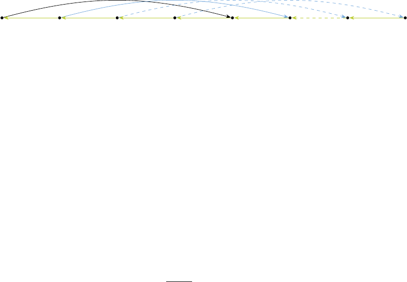
unmatched. In the latter case, by using (1), we must get λ
′′′′
satisfying (⋆) in at most
two additional steps, so that S(λ
′′′′
) ≤ S(λ
′′′
) + 1 ≤ S(λ) + 4.
Since we are interested in showing an exponential lower bound for the convergence time,
we pessimistically assume that whenever a stabilizing blocking pair is satisfied, the newly
obtained matching λ
′
moves four stable pairs towards stability, compared to original λ, and
preserves the condition (⋆).
Based on the previous analysis, we can obtain a lower bound on the number of steps
needed to reach S(µ) = n by considering the biased random walk S = S(λ)
k k + 1 k + 2 k + 3 k + 4 k + 5
n − 1
n
w.p. 1
on the set {k, k + 1, . . . , n}, with k ≡ ⌈(1 − ϵ)n⌉, defined as follows. It starts at k and
terminates when it reaches n; if S(λ) ever drops below k, we wait for it to return to that
value and restart the random walk. If our “starting” matchings do not satisfy (⋆), they
must satisfy it in at most four steps—in at most three, by our previous analysis, so here
again we bound the convergence time below—and we pessimistically assume they move with
probability one four stable pairs towards stability, i.e. S → S + 4. For all other nodes
between k and n, the condition (⋆) is satisfied, and we can either move one stable pair away
from stability (for destabilizing blocking pairs), S → S − 1, with the probability of
p
d
=
η − ϵ
η + ϵ
→ 1 as ϵ → 0,
or move four stable pairs towards stability (for stabilizing blocking pairs), S → S + 4, with
the remaining probability of
p
s
≡ 1 − p
d
→ 0 as ϵ → 0,
The rest of the proof is similar to Ackermann et al. (2011), and thus is omitted. It shows
41

that with high probability it takes at least exponentially many steps to reach S(µ) = n in
the biased random walk above.
Next, we present a sequence of markets satisfying the conditions of Proposition 1. For
simplicity of exposition, consider the following two markets of size n = 5 (on the left) and
n = 6 (on the right):
4, 5 3, 4 2, 5 5, 2 1, 1
1, 4 4, 3 3, 4 2, 5 5, 2
1, 3 5, 2 4, 3 3, 4 2, 5
1, 2 2, 5 5, 2 4, 3 3, 4
1, 1 2, 1 3, 1 4, 1 5, 3
and
4, 6 3, 5 2, 6 6, 2 5, 3 1, 1
1, 5 4, 4 3, 5 2, 6 6, 2 5, 3
1, 4 5, 3 4, 4 3, 5 2, 6 6, 2
1, 3 6, 2 5, 3 4, 4 3, 5 2, 6
1, 2 2, 6 6, 2 5, 3 4, 4 3, 5
1, 1 2, 1 3, 1 4, 1 5, 1 6, 4
,
each with its unique stable matching µ(f
i
) = w
i
, for any i ∈ [n].
For each market, it is straightforward to check that any f ̸= f
n
is preferred by ⌈n/2⌉ − 1
workers to their stable partners. In addition, any w ̸= w
1
is preferred by ⌊n/2⌋ − 1 firms to
their stable partners.
It is easy to generalize these two markets and their structure to arbitrary n, both odd
and even (the precise preferences are omitted and available upon request). By doing so,
we can construct a sequence of markets such that every agent a /∈ {f
n
, w
1
} is preferred by
approximately half of agents from the other side to their stable partners.
Equipped with this sequence of markets and Proposition 1, we are ready to prove the
main result. Consider any sequence of markets of size n ∈ N and any δ > 0.
For any market (of size n) in the sequence, we construct its extended version as follows.
Add new firms and new workers with preferences over each replicating the market of size
⌊δn⌋ constructed above. In addition, assume that all new firms (workers) prefer all original
workers (firms) over all newly added workers (firms). In contrast, all original firms (workers)
42

prefer all original workers (firms) over all new workers (firms).
The constructed market is indeed δ-augmented of size at most (1 + δ)n. Furthermore,
any agent on one side except one is preferred by at least η-proportion of agents from the
other side to their stable partners, for some η > 0 that does not depend on n.
Then, the desired result follows by similar arguments as in Proposition 1. Indeed, even
though now we consider the sequence of δ-augmented markets, their market sizes are still
increasing linearly, so the same result applies.
References
Abdulkadiroğlu, Atila and Tayfun Sönmez, “School Choice: A Mechanism Design
Approach,” American Economic Review, 2003, 93 (3), 729–747.
Ackermann, Heiner, Paul W Goldberg, Vahab S Mirrokni, Heiko Röglin, and
Berthold Vöcking, “Uncoordinated Two-Sided Matching Markets,” SIAM Journal on
Computing, 2011, 40 (1), 92–106.
Balinski, Michel and Guillaume Ratier, “Of Stable Marriages and Graphs, and Strategy
and Polytopes,” SIAM Review, 1997, 39 (4), 575–604.
Boudreau, James W, “A Note on the Efficiency and Fairness of Decentralized Matching,”
Operations Research Letters, 2011, 39 (4), 231–233.
Chen, Yi-Chun and Gaoji Hu, “Learning by Matching,” Theoretical Economics, 2020,
15 (1), 29–56.
Chung, Kim-Sau, “On the Existence of Stable Roommate Matchings,” Games and Eco-
nomic Behavior, 2000, 33 (2), 206–230.
Diamantoudi, Effrosyni, Eiichi Miyagawa, and Licun Xue, “Random Paths to Sta-
bility in the Roommate Problem,” Games and Economic Behavior, 2004, 48 (1), 18–28.
43
Eeckhout, Jan, “On the Uniqueness of Stable Marriage Matchings,” Economics Letters,
2000, 69 (1), 1–8.
Fernandez, Marcelo Ariel, Kirill Rudov, and Leeat Yariv, “Centralized Matching
with Incomplete Information,” American Economic Review: Insights, 2022, 4 (1), 18–33.
Gale, David and Lloyd S Shapley, “College Admissions and the Stability of Marriage,”
The American Mathematical Monthly, 1962, 69 (1), 9–15.
Gusfield, Dan, “Three Fast Algorithms for Four Problems in Stable Marriage,” SIAM
Journal on Computing, 1987, 16 (1), 111–128.
Inarra, Elena, Concepcion Larrea, and Elena Molis, “Random Paths to P-Stability in
the Roommate Problem,” International Journal of Game Theory, 2008, 36 (3), 461–471.
Klaus, Bettina and Flip Klijn, “Paths to Stability for Matching Markets with Couples,”
Games and Economic Behavior, 2007, 58 (1), 154–171.
Knuth, D. E., Marriages Stables, Les Presses de l’université de Montréal, 1976.
Kojima, Fuhito and M Utku Ünver, “Random Paths to Pairwise Stability in Many-to-
Many Matching Problems: a Study on Market Equilibration,” International Journal of
Game Theory, 2008, 36 (3), 473–488.
Lazarova, Emiliya and Dinko Dimitrov, “Paths to Stability in Two-Sided Matching
under Uncertainty,” International Journal of Game Theory, 2017, 46 (1), 29–49.
Manlove, David, Algorithmics of Matching under Preferences, Vol. 2, World Scientific,
2013.
McKinney, C Nicholas, Muriel Niederle, and Alvin E Roth, “The Collapse of a
Medical Labor Clearinghouse (and Why Such Failures Are Rare),” American Economic
Review, 2005, 95 (3), 878–889.
44

McVitie, D. G. and L. B. Wilson, “Stable Marriage Assignment for Unequal Sets,” BIT,
September 1970, 10 (3), 295–309.
McVitie, David G and Leslie B Wilson, “The Stable Marriage Problem,” Communica-
tions of the ACM, 1971, 14 (7), 486–490.
Millán, Beatriz and Eliana Pepa Risma, “Random Path to Stability in a Decentralized
Market with Contracts,” Social Choice and Welfare, 2018, 51 (1), 79–103.
Pittel, Boris, “The Average Number of Stable Matchings,” SIAM Journal on Discrete
Mathematics, 1989, 2 (4), 530–549.
Roth, Alvin E, “The Economist as Engineer: Game Theory, Experimentation, and Com-
putation as Tools for Design Economics,” Econometrica, 2002, 70 (4), 1341–1378.
Roth, Alvin E. and John H. Vande Vate, “Random Paths to Stability in Two-Sided
Matching,” Econometrica, 1990, 58 (6), 1475–1480.
and Marilda A. Oliveira Sotomayor, Two-Sided Matching: A Study in Game-
Theoretic Modeling and Analysis Econometric Society Monographs, Cambridge: Cam-
bridge University Press, 1992.
Roth, Alvin E and Xiaolin Xing, “Jumping the Gun: Imperfections and Institutions Re-
lated to the Timing of Market Transactions,” American Economic Review, 1994, pp. 992–
1044.
Tamura, Akihisa, “Transformation from Arbitrary Matchings to Stable Matchings,” Jour-
nal of Combinatorial Theory, Series A, 1993, 62 (2), 310–323.
Tan, JJ and WC Su, “On the Divorce Digraph of the Stable Marriage Problem,” Proc.
National Science Council, Republic of China, 1995, 19, 342–354.
45
