
e Census Place Project: A Method for Geolocating
Unstructured Place Names
Enrico Berkes
∗
Ezra Karger
†
Peter Nencka
‡
April 5, 2022
Researchers use microdata to study the economic development of the United States and the causal
eects of historical policies. Much of this research focuses on county- and state-level paerns
and policies because comprehensive sub-county data is not consistently available. We describe
a new method that geocodes and standardizes the towns and cities of residence for individuals
and households in decennial census microdata from 1790–1940. We release public crosswalks
linking individuals and households to consistently-dened place names, longitude-latitude pairs,
counties, and states. Our method dramatically increases the number of individuals and house-
holds assigned to a sub-county location relative to standard publicly available data: we geocode
an average of 83% of the individuals and households in 1790–1940 census microdata, compared
to 23% in widely-used crosswalks. In years with individual-level microdata (1850–1940), our av-
erage match rate is 94% relative to 33% in widely-used crosswalks. To illustrate the value of our
crosswalks, we measure place-level population growth across the United States between 1870 and
1940 at a sub-county level, conrming predictions of Zipf’s Law and Gibrat’s Law for large cities
but rejecting similar predictions for small towns. We describe how our approach can be used to
accurately geocode other historical datasets.
∗
e Ohio State University, [email protected]du
†
Federal Reserve Bank of Chicago, [email protected]
‡
Miami University, [email protected]
We thank IPUMS, Ancestry.com, and FamilySearch for providing us with access to data for use in this paper.
We also thank participants at the Methodological Advances in the Extraction and Analysis of Historical Data and
Southern Economic Association conferences for their helpful feedback. Any views expressed in this paper do not
necessarily reect those of the Federal Reserve Bank of Chicago or the Federal Reserve System.
1

1 Introduction
e public release of full-count decennial census microdata from 1790-1940 has increased the
quantity and quality of research studying trends and policies in the United States during these
periods. Much of this work uses state- or county-level data (e.g., Aaronson and Mazumder, 2011;
Donaldson and Hornbeck, 2016; Desmet and Rappaport, 2017) or focuses on a small number of
counties or large cities where researchers have detailed sub-county microdata (e.g., Michaels,
Rauch, and Redding, 2012; Shertzer, Walsh, and Logan, 2016; Brooks and Lutz, 2019; Fishback
et. al, 2020; Aaronson, Hartley, Mazumder, 2021). One reason for this geographic focus is data
availability: commonly-used historical datasets only consistently identify states, counties, and
large cities. However, states and counties cover broad geographic areas and contain important
heterogeneity in demographics, policies, and access to local amenities; while larger cities can be
systematically dierent from their smaller peers. In this paper, we use a new method to construct
consistent measures of place for U.S. residents in the 1790—1940 decennial censuses. We create
a crosswalk that allows researchers using public or restricted decennial census microdata to link
respondents to consistently dened sub-county locations.
1
To construct these links, we clean and analyze raw place names from census manuscripts
corresponding to cities and townships. Aer we identify all unique places within a given decade
of census microdata, we iterate through the strings to identify a standardized location name and
latitude/longitude. To do this, we match strings to geocoded places in NHGIS historical place
point les, GNIS place les, and Google Maps.
2
When location strings are not reported or found,
we are oen able to exploit the existence of nearby enumeration districts to impute an accu-
rate sub-county location. Aer we perform these steps for every census year in our sample, we
standardize place names and locations across years to make our locations temporally consistent.
1
We dene a sub-county location as any location at a ner geography than county borders, not ocial Census
sub-county areas.
2
For more details about NHGIS place point les, see Manson et al. (2021). For more details about the GNIS place
les, see United States Geological Survey (2021).
2

Relative to publicly available datasets, we map many more people to sub-county locations.
We match an average of 83% of the individuals and households in 1790–1940 census microdata to
the longitudes and latitudes of their cities and towns of residence, compared to 23% in currently
widely-used crosswalks. In years with individual-level microdata (1850–1940), our average match
rate is 94% relative to 33% in widely-used crosswalks. In 1870 (the year where we obtain our best
match rate), we geocode 99.1% of individuals relative to 19% in public crosswalks.
We highlight the value of our new place data with two applications. First, we take the 69,393
unique geocoded places from our census microdata crosswalks covering 1790-1940 and we it-
eratively cluster these places into 42,133 consistently-dened places over time. Our clustering
approach is informed by the closeness and size of neighboring places and addresses the fuzziness
of xed place denitions both over time and across borders. Our clusters account for shiing
place borders, annexations, subsumed suburbs, and ghost towns. We include these clusters as
variables in our crosswalks, providing other researchers with a data-driven denition of local
metropolitan areas.
Next, we link our clusters to census microdata and create granular measures of place-level
population growth over time. We show that our clustered places consistently follow Zipf’s Law
and Gibrat’s Law for large cities in historical time periods, matching predictions from theory
and modern-day empirical contexts (e.g., Gabaix 1999; Ioannides and Overman 2003; Giesen and
Sudekum, 2011). We also nd sharp deviations from Zipf’s Law and Gibrat’s Law for small places.
To the best of our knowledge, we are the rst to document these paerns for smaller places
across the entire U.S. in a historical context, since prior historical work focuses only on large
cities, county-level paerns (eg. Desmet and Rappaport, 2017), or a small subset of states with
high-quality sub-county data (Michaels, Rauch, and Redding, 2012).
3
Our work builds on past eorts to digitize, standardize, and improve the usability of the com-
plete count census les. In particular, IPUMS sta have standardized large portions of the histor-
3
For a review of prior historical work on city growth rates in a historical context, embedded in a larger discussion
of historical urban economics, see Hanlon and Heblich (2021).
3

ical census enumeration sheets and created variables for many common elds that researchers
commonly use (Ruggles et. al, 2021). Public IPUMS data generally identies only larger cities,
though the eective city-size thresholds vary over time.
4
Our approach is informed by eorts
like the Census Linking Project, which provides public census data users a crosswalk that allows
them to link census respondents across time, a process that otherwise would require access to
restricted census data (Abramitzky, Boustan, and Rashid, 2020).
Many papers (including our own prior work) use raw census strings to dene sub-county
areas that are smaller than IPUMS-provided cities for subsets of the historical censuses.
5
For ex-
ample, Karger (2021) and Berkes and Nencka (2021) develop string cleaning methods to identify
small cities and towns that had Carnegie libraries in the early 1900s. Michaels, Rauch, and Red-
ding (2012) standardize sub-county areas in the 1880 census and link these areas to 2000 data to
study long-run trends in population dynamics.
6
Nagy (2020) standardizes cities in the 1790 to
1860 censuses to study city formation and the eects of transportation infrastructure. Feigen-
baum and Gross (2021) clean city names with more than 2,000 people from 1910 to 1940 to track
information on telephone operators. Oerstrom, Price, and Van Leeuwen (2021) use linked cen-
sus records from 1900–1940 to measure changes in city population size for the 1,000 largest cities
in 1900. Connolly (2021) digitizes locations in the 1920 census to study the impact of two-year
colleges on children’s adult outcomes. To our knowledge, we are the rst to standardize raw loca-
tion strings for the universe of all available full-count census data, allowing us to use information
across census years to improve the accuracy of matches. Moreover, we identify additional sub-
county locations for observations with missing or uninformative strings by relying on nearby,
sequentially numbered enumeration districts. Finally, by releasing our crosswalks and associ-
4
See the IPUMS documentation for a detailed description of the IPUMS CITY variable, which is the primary
temporally consistent source of sub-county place information in publicly available Census microdata. We describe
the IPUMS standardization more fully and compare our mapping to theirs in Section 3.1. For 1940, IPUMS recently
released a more comprehensive city variable that captures more (but not all) of the locations that we geocode. is
variable is named PLACENHG in the public 1940 data and is constructed using NHGIS place les.
5
It would be dicult to highlight every paper that used sub-county historical variation. In this section, we
highlight a number of illustrative examples.
6
ese areas are also used in Hodgson (2018) to study the eects of the railroad on population growth.
4

ated time-consistent clusters, we give all researchers the ability to study sub-county trends and
policies while reducing duplicated eort in the research community.
Relative to publicly released census data, our added value is highest when studying rural ar-
eas or smaller locations adjacent to nearby cities. By contrast, we do not aempt to geocode
within-city locations like addresses or neighborhoods, which are the subject of recent valuable
exercises focused on larger cities (e.g., Logan et. al 2011, Shertzer, Walsh and Logan, 2016; Fish-
back et. al, 2020; Brooks and Lutz, 2019; Aaronson, Hartley, Mazumder, 2020). Sub-city geocoding
requires historically accurate street layouts, which makes it dicult to apply to smaller or rural
areas. In recent work, Ferrara, Testa, and Zhou (2022) construct population-based crosswalks of
countries and congressional districts using backward-looking population projections. Our work
complements their contribution: we focus on matching individuals to geocoded places using con-
temporaneous location information, allowing researchers to use individual microdata to measure
area characteristics. We do not aempt to model the entire geographic population distribution.
7
While our focus is historical U.S censuses, our methods apply more broadly. Our publicly-
accessible programs provide a consistent and automatic methodological approach to geocoding
and clustering townships, cities, and unincorporated places. We hope that these methods will
be useful in other contexts where researchers need to assign geocodes to historical documents
that contain location strings. For example, U.S patents include the city, state, and county of
inventors, and birth certicates oen include detailed birth locations. Our methods provide an
easily applicable framework for geocoding locations in these documents.
e rest of the paper is structured as followed: in Section 2 we discuss our geocoding proce-
dure. In Section 3 we compare our geocode coverage to existing census data and show an illus-
trative example of how to use our data. In Section 4 we discuss how to implement our method in
other applications which involve sub-county data. In Section 5 we conclude.
7
Ferrara, Testa, and Zhou (2022) discuss both the benets and limits of their approach in Section 4 of their paper.
5

2 Method
In this section, we describe the method that we use to geocode the historical censuses. We discuss
our approach with reference to the information available in in the US census, though as we discuss
in Section 4 many of the steps below will be similar for any data involving historical locations.
We begin by identifying all the geographic information available in IPUMS’ raw decennial
census data from 1790–1940. ese variables represent raw text strings and in some cases IPUMS-
standardized place names. e data includes between one and six raw location strings each year
along with contemporary county and state identiers.
8
ese text strings are sometimes broad
(eg. “New York City”), but oen contain granular information about places (eg. “District 83, Beebe
Volborg”).
We clean the text strings by applying a standardized set of criteria, described in more detail in
our Data Appendix. To summarize these steps, we standardize common prexes, remove punc-
tuation, remove common words (like “justice ward” or “courthouse”), and standardize cardinal
directions when they refer to an explicit quadrant of a town or city. For example, the text string
“Precinct 10, Aubrey [30] & Precinct 6, South Side [11]” is cleaned into the location “Aubrey.”
Next, we aempt to geocode all of our clean place names in several steps, relying on histor-
ical spatial databases from IPUMS National Historical Geographic Information System (NHGIS)
and e Geographic Names Information System (GNIS). NHGIS contains the locations of incor-
porated and unincorporated places used by the U.S. Census Bureau from 1900 onward. GNIS is
the U.S. Board on Geographic Names’ consistent database of places, maintained by the federal
government. We iterate over the raw census location strings, starting with the most granular
place name and then using less granular place names if we cannot make a match.
For 1900–1940, we take each cleaned census place and its associated county in historical data,
and we look for the most similarly named place in NHGIS that is in the correct historical county.In
most cases, we use county and state maps corresponding to the relevant census year. However,
8
For a full list of the variables we use, see our Data Appendix.
6

we have a penultimate round of matching that uses 1910 counties as our reference geography.
e standardized census data uses some county or state names before they were ocial (e.g.,
West Virginia in 1860). is additional step reduces false negative matches. We require that the
census and NHGIS strings have a match score of 0.95 to identify accurate matches.
9
If we cannot
nd a match, we then perform the same search within the GNIS place data, looking for matches
to dierent feature types, ranging from populated places to post oces and valleys. For any
unmatched census places aer this step, we search NHGIS and then GNIS for place names in the
correct county that have an edit-distance of 1 with our census place. Finally, we remove cardinal
directions and look again for places in the NHGIS and GNIS les with a match score of 0.95.
Our strategy for geocoding the 1790–1880 census years is similar to our process for 1900-1940.
However, since NHGIS historical place points are not available before 1900, we only use the GNIS
place le to match census strings to place names. Otherwise, we use identical approaches.
Once we have initial geocodes for all census years from the NHGIS and GNIS les, we com-
plete four nal steps to increase match rates and standardize geocodes. First, we impute coor-
dinates for places in enumeration districts when another named place within that enumeration
district was successfully geocoded. Second, we impute coordinates for enumeration districts that
are numerically between two successfully geocoded, nearby enumeration districts. ird, we
search Google Maps for all unmatched places. We use the Google Maps latitude and longitude if
it falls within the correct historical census county. Lastly, we compare across census years and
standardize the spelling of matched place names and the exact coordinates of each place. is
standardizes small perturbations in the reported coordinates of places across NHGIS, GNIS, and
Google Maps. In our crosswalks, we include ags that indicate at which step each match is made,
so that researchers can exclude these imputed matches as desired. e Data Appendix includes
more details on all of these steps.
Aer this procedure, there are 708,928 unique census year -by- cleaned location observations
9
e match score is calculated using the string-matching process of the fuzzywuzzy library in Python. It combines
several methods for calculating a measure of ‘distance’ between potential strings, normalizing by string length.
7
that we extract from the raw census data. Of those year-place observations, we fail to geocode
42,155 places (6% of the total number). 390,913 places (55%) match to NHGIS places in our rst
aempt, and an additional 198,491 (28%) match to the most common types of GNIS places in our
rst aempt. 14,690 (2%) match to NHGIS and GNIS places using slight variation in fuzziness of
match requirements, and an additional 54,403 (8%) match through our two enumeration district
imputation steps. By ensuring time-consistency of identically-named place names across census
years, we geocode an additional 7,357 (1%) of places. And lastly, we geocode 919 (0.2%) of places
using Google Maps.
Our nal crosswalks create consistent longitudes and latitudes of each person’s town, city,
or unincorporated place of residence. To increase the usability of our crosswalks, we also assign
modern-day county and state identiers to each geocoded place. is provides a consistent mea-
sure of county and state of residence for all geocoded observations. Our crosswalks provide an
accurate and consistent way to identify the county of residence for the vast majority of U.S. res-
idents, complementing recently-constructed spatial harmonizations of changing county borders
over time (Hornbeck, 2010; Perlman, 2014; Ferrara, Testa, and Zhou, 2022).
3 Results and Application
3.1 Geocoding Rates
In this subsection, we describe the coverage of our geocoded data across decades and compare
our match rates to existing public data. In all years, our match rates allow researchers to observe
more sub-county locations relative to previously available sources. To see this, we calculate the
share of observations in public census data that can be geocoded using extracts from IPUMS.
In particular, we compare our cities to observations with non-missing IPUMS standardized city
variables “CITY” or (for 1940 only) “PLACENHG.”
We show our match rate comparison in Figure 1, which plots the percent of census observa-
8

tions with valid sub-county locations across years, for both our crosswalks and publicly available
IPUMS data. We successfully match 56-99 percent of observations to a sub-county location, de-
pending on the census year. Our match rate generally increases over time, particularly when
the census moves to the collection of individual-level data in 1850. Match rates surpass 91% in
all years from 1860–1940.
10
Our match rate diers across years due to the various methods that
censuses used to collect information on geographical locations. For example, the 1870 census
has signicantly more geographical digitized information relative to prior years. In most cases,
our failure to link a sub-county location to a valid latitude and longitude occurs when there is
no geographical information beyond county recorded on an enumeration district and we have
limited information on adjoining enumeration districts.
11
3.2 Example: Waukesha County
To illustrate the value of our data and approach, consider Waukesha County in Wisconsin. Today,
Waukesha County is Wisconsin’s third-largest county by population and covers 581 square miles.
e county is geographically diverse: its eastern portion is an extended suburb of Milwaukee
and is heavily commercialized with manufacturing and service industries, while the western and
southern portions are rural and contain signicant farmland.
In 1930, Waukesha County had 52,000 people. In publicly available 1930 census data, the
only available sub-county location is the county seat, Waukesha.
12
In 1930, the city of Waukesha
contained roughly 35% of the county population, leaving 65% of the city lacking a valid sub-
county location. By contrast, we assign 100% of the 1930 Waukesha County population to a valid
10
An observation is a household in 1790-1840. Starting in 1850, an observation is a person. We focus on census
observations and not the count of people throughout this paper because the decennial population censuses did not
collect information about the slave population in all years.
11
Conceptually, it is possible to map these places manually by consulting the original enumeration district maps,
as is done by Connolly (2021) for a set of 1920 cities. Unfortunately, since enumeration district boundaries change
over time, this procedure would need to be repeated for every decade in our sample. ese unnamed locations tend
to be small rural areas.
12
is location starts to be identied in the public census microdata from IPUMS in 1900. Before this, there is no
city identied in this county in the public census data.
9

sub-county location.
13
In Figure 2, we illustrate the coverage of our geocoded 1930 places using a map of modern-
day Waukesha County locations. e city of Waukesha—framed in black—is the only sub-county
1930 location in public census data. By contrast, all of the cities highlighted in blue are also
included in our new geolocated place data. is includes extremely small locations in 1930—for
instance, Wales had only 123 residents, while Dousman had 256 residents. Figure 2 highlights that
our new data shows the geographic diversity of Waukesha County. Even in 1930, the jobs and
industries of the eastern portions of the county were changing and becoming more industrialized
relative to the more rural parts of the county. With our location data linked to publicly-available
IPUMS data, researchers can observe and study the persistence of these within-county dierences
throughout history.
3.3 Clustering
While our place-level longitude-latitude mappings are comprehensive, these places are not de-
ned consistently over time. To address this limitation, we use an iterative density-clustering
approach to map our 69,393 unique locations across the 150 year period of 1790–1940 to a smaller
set of 42,133 consistently-dened places. While most places are distinct and not combined in this
step, larger cities like Atlanta, Pisburgh, and Chicago have borders that expand over time as
they merge with other towns and experience high levels of in-migration. Our method captures
these expanding borders, allowing us to consistently measure features of these cities over time.
14
13
Our match rates for this example are similar if we focus on other census years with individual microdata. In 1940,
IPUMS data also captures some of these sub-county locations with their newly constructed “PLACENHG” variable.
14
We cluster places consistently over time so that researchers can use our cluster identiers to track city growth,
shrinking urban borders, mergers, and annexation. For example, in 1907 Pisburgh annexed nearby Allegheny City
against the wishes of a majority of Allegheny residents who, in repeated referenda, rejected the annexation aempt.
e annexation was forced on Allegheny by Pennsylvania, whose legislators passed a law allowing a majority of the
combined voters from Pisburgh and Allegheny City to determine the results of the annexation, even if a majority
of the voters in the targeted city (Allegheny City) rejected the annexation aempt. For more discussion of this and
related annexations, see Lonich (1993). Researchers interested in the distinction between Pisburgh and Allegheny
City can use our data to dierentiate those two places in years where the places were enumerated distinctly. But
as the cities merged, the denition of Pisburgh and Allegheny became amorphous, and our clusters provide a
10

We iteratively cluster any neighboring places that are within three miles of each other within
census years and across census years. We also cluster together any two places i and j that are
within 100 ∗ K
cluster
∗ max{sharepop
i
, sharepop
i
} miles of each other, where sharepop
i
is the
fraction of the population in decennial census data that we map to place i across all years (1790–
1940), assigning equal weight to each year. For our main results, we rely on a constant K
cluster
of 5. is choice of clustering allows large cities to be combined with more of their suburbs. For
example, Chicago contains roughly 2.5% of the people in decennial census microdata from 1790-
1940. When K
cluster
= 5, Chicago will be close neighbors with any smaller place within 12.5
miles of it. We cluster places consistently over time by dening each cluster to be the connected
component of all close neighbors for each place.
In Figure 3, we map all of our consistently dened places. We color each cluster to reect close
neighbors. Our individually-geocoded places reect the geographic distribution of people in the
United States from 1790–1940, highlighting the densely populated New England corridor. Our
clusters show consistently-dened metropolitan areas that can spread across state and county
borders. We include these cluster denitions in our crosswalks so that other researchers can use
them.
To further show the value of our clusters, in Figure 4 we focus on four representative states
across dierent census regions and highlight the individual geocoded places, our consistently-
dened clusters, and the ve largest clusters in each state. e top le panel shows that our
clustering combines the Birmingham, Alabama suburbs into one cluster. In the top right panel,
Miami and Tampa Bay, Florida are combined into distinct clusters with their nearby suburbs. In
the boom panels, the dense west coast of Oregon is clustered into a small number of metropoli-
tan areas. In Pennsylvania, Pisburgh and Philadelphia form distinct clusters.
15
In Figure 5, we show the same four states with modern-day county borders. ese maps show
the value of our geocoded places to researchers hoping to analyze spatial variation in access
time-consistent approach to measuring the number and type of people living in the Pisburgh area over time.
15
Figures A1–A4 show full-page versions of these state-level gures for easy readability.
11

to policies or spatial outcomes in a historical seing. We geocode an average of 23 places per
modern-day county in the U.S. is granular classication of locations gives researchers the tools
to analyze distance-based access to local programs, within-county border discontinuity designs,
and urban/rural migration paerns within counties.
16
Our preferred value of K
cluster
in the above specications is 5 because that allows large cities
to subsume close suburbs, but it maintains the geographic distinctness of nearby small places. We
also provide alternative clusters for dierent values of K
cluster
so that researchers can choose that
clustering that best t their analysis based on the level of geographical variation in which they
are interested. In Figure 6, we show our clusters for Washington with two levels of aggregation:
K
cluster
= 5 and K
cluster
= 500. With the less aggressive level of aggregation, Seale and Evere
(29 miles away from each other) form distinct clusters with their respective surrounding suburbs
and nearby towns. With more aggressive clustering (K
cluster
= 500), the Seale and Evere
clusters merge and become one larger Seale metropolitan area and the Spokane cluster absorbs
more nearby towns.
3.4 Population Dynamics
To showcase our new crosswalks, we use our preferred clustered places to examine the size dis-
tribution of historical places in the U.S. and place-specic population growth. A large literature
in urban economics models and empirically quanties the formation and growth of cities. is
literature focuses on two ‘laws’: Zipf’s Law, which states that there is a linear relationship at the
city-level between log(population) and log(rank) of population, and Gibrat’s Law, which states
that the population growth rate is independent of city size. Gabaix (1999) showed that if a set of
cities grow independently of initial city size, following Gibrat’s Law, then the steady-state size
distribution will follow Zipf’s Law. Testing these predictions using high-quality historical data
gives urban economists the ability to evaluate theories of long-run city population dynamics.
16
Figures A5–A8 show full-page versions of these state-level gures for easy readability.
12

We use our geocoded historical places to evaluate these two laws. In Figures 7 (for 1870
places) and 8 (for 1940 places), the top panel shows the relationship between log(population)
and log(rank) for IPUMS-dened cities and the boom panel shows the same relationship for
our geocoded places. We focus on places with populations over 20,000. In the IPUMS-based top
panels, there is a deviation from Zipf’s Law at the right tail of the city size distribution in both 1870
and 1940—the most populous cities look smaller than what Zipf’s Law predicts if we use IPUMS’s
city classication. In the boom panel of each gure, we plot the same log(population)-log(rank)
graph with our geocoded and clustered places. Using our places, we match the predictions of
Zipf’s Law almost exactly. Our decision to cluster places combines large cities with their suburbs,
and these clustered places match the predictions of Zipf’s Law.
In Figures 9 and 10, we extend Zipf’s Law to all tracked places in 1870 and 1940 respectively.
In the top panels, we show the IPUMS-based log(population)-log(rank) plot and in the boom
panels, we present the log(population)-log(rank) plot for all of our geocoded clusters. In both
years (1870 and 1940), we see sharp deviations from Zipf’s Law for places with fewer than 500
residents in our geocoded data. Focusing on the smallest places, we see that they are underrep-
resented in our sample of places relative to the predictions of Zipf’s Law. In 1870, we do not see
a similar paern in IPUMS’s data because the publicly available crosswalks do not contain the
locations of small cities and towns. In 1940, when IPUMS coverage is higher, we do see the same
deviation from Zipf’s Law for smaller cities and towns.
In Figure 11, we compare the prediction of Gibrat’s Law in IPUMS’ city data (panel A) and
our geocoded clusters (panel B). We focus on place-level population growth from 1870 to 1940 for
places with populations less than 50,000 in 1870.
17
IPUMS consistently tracks very few cities over
this time period, but for the 144 cities with a population over 10,000 in 1870, we see a close match
to the predictions of Gibrat’s Law–city growth from 1870 to 1940 seems uncorrelated with the
17
e results are unchanged if we include the largest cities, but including the largest cities in the panels makes
it more dicult to see the non-monotonic population growth rate dynamics for cities with lower initial population
levels in 1870.
13
initial 1870 population. Cities of all sizes quadrupled in size between 1870 and 1940. But in our
geocoded places we see a strikingly dierent conclusion. We show that population growth rates
were U-shaped over this 70-year period. e population of smaller places grew almost nine-fold
on average while the population of the largest places more than quadrupled. But for mid-sized
places with populations around 1,000 people, we see much smaller growth rates around 150%.
is is a paern that also exists at the county level, as shown by Desmet and Rappaport (2017).
We are the rst to show these historical paerns at the town and city level for all places in the
United States.
4 Discussion and application to additional datasets
So far, we have discussed our method and applications exclusively in the context of the historical
US decennial censuses. However, much of the code that we release can be used to geocode other
sources of historical data. In addition, the steps that we use can serve as a conceptual guide for
other researchers. However, like all methodological contributions, our approach will apply very
well in some cases and less well in others. In this subsection we discuss these tradeos.
Our current code is optimized to geocode historical US cities and townships. It is most eas-
ily applied to other documents that contain the same level of geographic detail. Two important
examples are patent documents and birth/death certicates. Both typically contain the city of
the invention or event, and both — because of the limits of modern OCR soware — are oen
measured with some error. Our code can clean these location strings and fuzzily match them
to historically accurate geocoded places. All that is required as an input is a vector of possible
strings for each document. Since our code was developed using US census data, it may need to
be modied: For example, in the censuses there are predictable strings that need to be cleaned
before geocoding (e.g., “WARD”, “DISTRICT”). To the extent that dierent datasets contain dif-
ferent strings that need cleaning, this code should be adjusted. Otherwise, our procedure has few
14
census-specic steps.
By contrast, because of our seing our code cannot directly geocode sub-city US data (e.g.,
streets or blocks) or locations outside the US. However, with appropriate changes, the structure of
our code could be used in these cases. For example, to geocode streets, one could take information
on raw streets in the censuses, clean them using our algorithms, and match them to contemporary
street databases (instead of NHGIS/GNIS place points). Similarly, our approach and code can be
generalized to other countries, though many methodological choices will need to be made as a
function of the underlying strings and location databases available for that country.
Beyond our code, our geocoded census locations can also be used in methodological projects.
For example, researchers linking birth certicates to decennial census microdata face the lim-
itation that within a state or county, there can be multiple people with similar names. Using
our geocoded sub-county locations to aid in those links can increase match rates and lower false
positive rates.
5 Conclusion
Researchers oen use place-level data to measure the causal eects of local policies and to de-
scribe historical trends. ese analyses are oen done at the county- or state-level because it is
challenging to link individuals to consistently dened local places across census years. In this
paper, we describe and release public crosswalks linking the vast majority of 1790-1940 census
respondents to longitudes and latitudes. ese crosswalks allow analysts to explore sub-county
research questions and trends using public census data.
We present two applications of our crosswalks to demonstrate their value. First, we iteratively
cluster geocoded places with close neighbors, producing a consistent denition of place. is
application addresses the common concern that regularly-updated county borders and shiing
municipal boundaries make it dicult to match and compare places over time. Second, we test
15
the predictions of Zipf’s Law and Gibrat’s Law in a historical context, nding clear deviations
from theoretical predictions about the city size and city growth distribution. While these ndings
have been observed in more aggregated data, we are the rst to illustrate these paerns over long
time periods with national data on “places”.
e most important application of this paper is the method itself. Researchers spend signi-
cant and oen-duplicated time standardizing common spatial datasets, particularly when work-
ing with historical sources. We hope that the process we present in this paper helps researchers
link other datasets that include unstructured place names—for example, patent data or birth and
death records—to sub-county geocodes.
16
References
[1] Aaronson, Daniel, and Bhashkar Mazumder. “e Impact of Rosenwald Schools on Black
Achievement.” Journal of Political Economy 119, no. 5 (2011): 821-888.
[2] Aaronson, Daniel, Daniel Hartley, and Bhashkar Mazumder. “e Eects of the 1930s HOLC
Redlining Maps.” American Economic Journal: Economic Policy 13, no. 4 (2021): 355-92.
[3] Abramitzky, R., Leah Boustan, and Myera Rashid. Census Linking Project: Version 1.0
[dataset]. 2020. Data retrieved from, hps://censuslinkingproject.org.
[4] Berkes, Enrico, and Peter Nencka. “Knowledge Access: e Eects of Carnegie Libraries on
innovation.” (2021).
[5] Brooks, Leah, and Byron Lutz. “Vestiges of Transit: Urban Persistence at a Microscale.” Review
of Economics and Statistics 101, no. 3 (2019): 385-399.
[6] Connolly, Kevin. “How Does Access to College Aect Long-Term Life Outcomes? Evidence
from U.S. Openings of Two-Year Public Colleges” (2021).
[7] Desmet, Klaus, and Jordan Rappaport. “e Selement of the United States, 1800–2000: e
Long Transition Towards Gibrat’s Law.” Journal of Urban Economics 98 (2017): 50-68.
[8] Donaldson, Dave, and Richard Hornbeck. “Railroads and American Economic Growth: A
“Market Access” approach.” e arterly Journal of Economics 131, no. 2 (2016): 799-858.
[9] Feigenbaum, James, and Daniel P. Gross. “Organizational Frictions and Increasing Returns
to Automation: Lessons from AT&T in the Twentieth Century.” Available at SSRN 3912116
(2021).
[10] Ferrara, Andreas, Patrick Testa, and Liyang Zhou. “New area-and population-based geo-
graphic crosswalks for US counties and congressional districts, 1790-2020.” Available at SSRN
4019521 (2022).
[11] Fishback, Price V., Jessica LaVoice, Allison Shertzer, and Randall Walsh. “Race, Risk, and the
Emergence of Federal Redlining” No. w28146. National Bureau of Economic Research, 2020.
[12] Gabaix, Xavier. “Zipf’s law for cities: an explanation.” e arterly Journal of Economics
114, no. 3 (1999): 739-767.
[13] Giesen, Kristian, and Jens S
¨
udekum. “Zipf’s law for cities in the regions and the country.”
Journal of Economic Geography 11, no. 4 (2011): 667-686.
[14] Hanlon, W. Walker, and Stephan Heblich. “History and Urban Economics” No. 27850. Na-
tional Bureau of Economic Research, 2021; accepted at Regional Science and Urban Economics.
17
[15] Hodgson, Charles. “e Eect of Transport Infrastructure on the Location of Economic Ac-
tivity: Railroads and Post Oces in the American West.” Journal of Urban Economics 104
(2018): 59-76.
[16] Hornbeck, Richard. “Barbed wire: Property rights and agricultural development.” e ar-
terly Journal of Economics 125, no. 2 (2010): 767-810.
[17] Ioannides, Yannis M., and Henry G. Overman. “Zipf’s Law for Cities: An Empirical Exami-
nation.” Regional Science and Urban Economics 33.2 (2003): 127-137.
[18] Karger, Ezra. “e Long-Run Eect of Public Libraries on Children: Evidence from the Early
1900s.” (2021).
[19] Logan, John R., Jason Jindrich, Hyoungjin Shin, and Weiwei Zhang. “Mapping America in
1880: e Urban Transition Historical GIS Project.” Historical Methods 44, no. 1 (2011): 49-60.
[20] Lonich, David W. “Metropolitanism and the Genesis of Municipal Anxiety in Allegheny
County.” Western Pennsylvania History: 1918-2018 (1993): 79-88.
[21] Michaels, Guy, Ferdinand Rauch, and Stephen J. Redding. “Urbanization and structural
transformation.” e arterly Journal of Economics 127, no. 2 (2012): 535-586.
[22] Nagy, D
´
avid Kriszti
´
an. “Hinterlands, City Formation and Growth: Evidence from the US
Westward Expansion.” (2020).
[23] Oerstrom, Samuel M., Joseph P. Price, and Jacob Van Leeuwen. “Using Linked Census
Records to Study Shrinking Cities in the United States from 1900 to 1940.” e Professional
Geographer (2021): 1-14.
[24] Perlman, Elisabeth R. (2014). Tools for Harmonizing County Boundaries [Computer so-
ware]. Retrieved from hp://people.bu.edu/perlmane/code.html.
[25] Ruggles, Steven, Sarah Flood, Sophia Foster, Ronald Goeken, Jose Pacas, Megan Schouweiler,
and Mahew Sobek. IPUMS USA: Version 11.0 [dataset]. Minneapolis, MN: IPUMS, 2021.
hps://doi.org/10.18128/D010.V11.0
[26] Shertzer, Allison, Randall P. Walsh, and John R. Logan. “Segregation and Neighborhood
Change in Northern Cities: New Historical GIS Data from 1900–1930.” Historical Methods: A
Journal of antitative and Interdisciplinary History 49, no. 4 (2016): 187-197.
[27] Steven Manson, Jonathan Schroeder, David Van Riper, Tracy Kugler, and Steven Ruggles.
IPUMS National Historical Geographic Information System: Version 16.0 [dataset]. Min-
neapolis, MN: IPUMS. 2021. hp://doi.org/10.18128/D050.V16.0.
[28] United States Geological Survey. “Geographic Names Information System”. Updated August
27, 2021. Accessed at hps://www.usgs.gov/core-science-systems/ngp/board-on-geographic-
names/download-gnis-data.
18
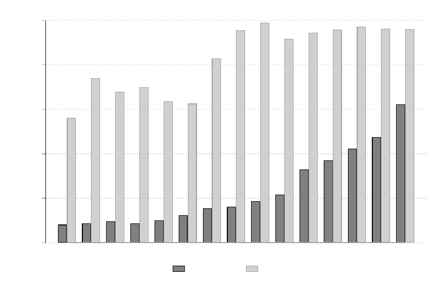
Figure 1: Census observations with valid sub-county locations, by data source and census year
0
.2
.4
.6
.8
1
Share of observations with valid sub−county location
1790 1800 1810 1820 1830 1840 1850 1860 1870 1880 1900 1910 1920 1930 1940
Public data CPP data
Notes: is gure shows the share of census observations with a valid sub-county location in each census year
separately for publicly available IPUMS census data and the newly constructed Census Place Project data. An
observation in 1790-1840 is a household. Starting in 1850, each observation is a non-slave member of the
household. e 1890 census manuscripts were lost in a re.
19
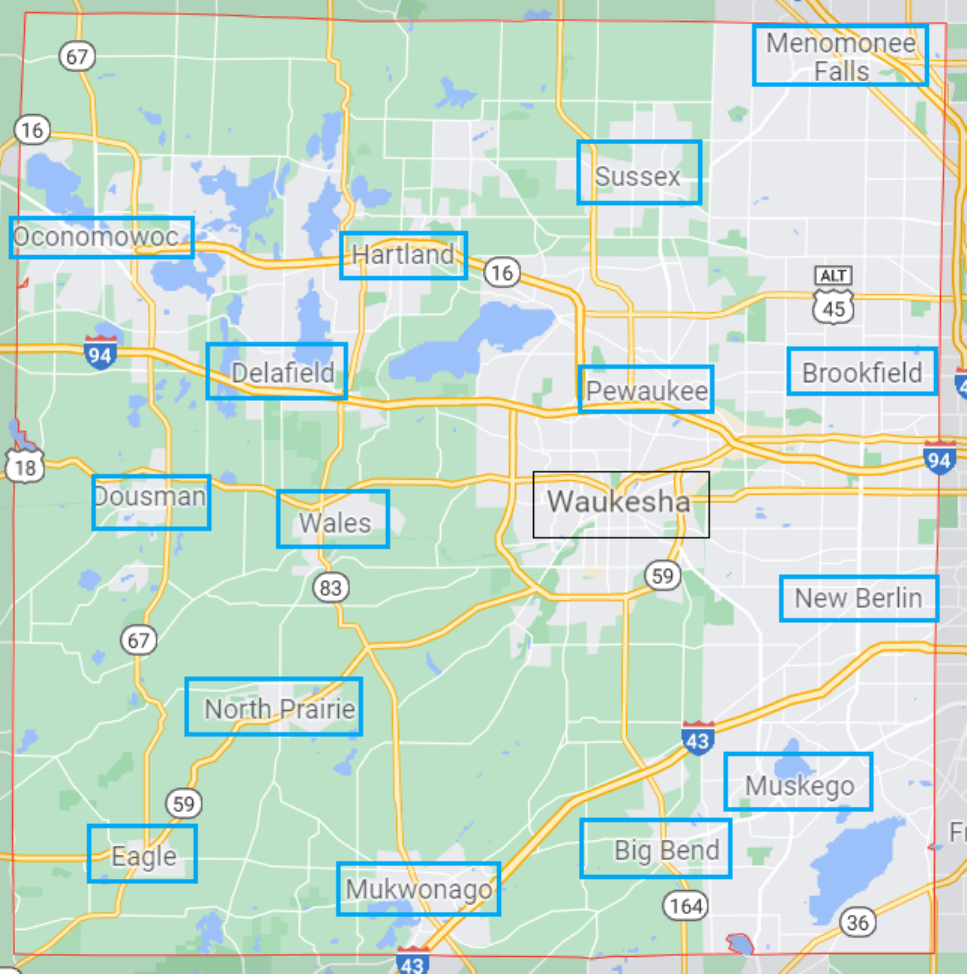
Figure 2: Waukesha County Wisconsin, modern map with 1930 census data coverage highlighted
Notes: is gure is a modern-day map of Waukesha County, accessed via Google Maps. Only the city of Waukesha
(highlighted in black) is identied in public 1930 census data. Our geocoded data identies all the cities highlighted
in blue, in addition to smaller areas not labeled on the map
20
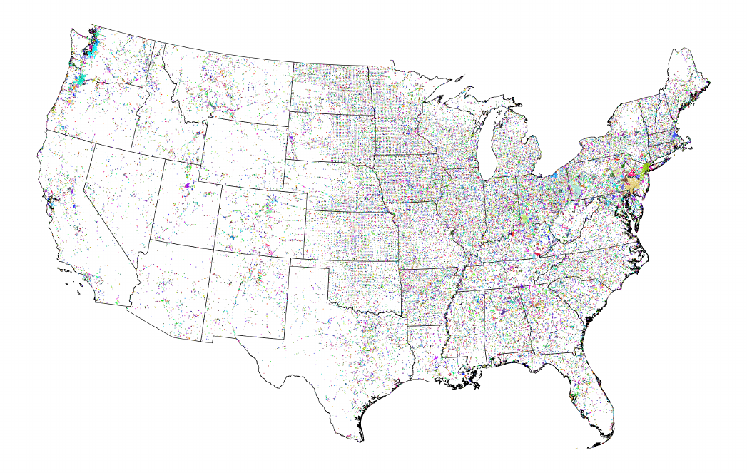
Figure 3: All clustered places
Notes: is gure maps all of our 69,393 unique places across the years 1790–1940 aer assigning the places to
consistent clusters (with K
cluster
= 5). Places within a cluster are given the same color, highlighting large colors
surrounding major metropolitan areas (like New York City).
21
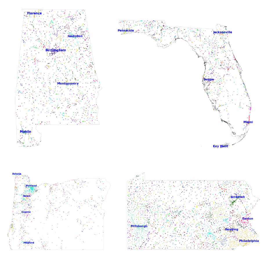
Figure 4: State-level maps of clustered places
Alabama Florida
Oregon Pennsylvania
Notes: is gure maps our geocoded places in four states: Alabama, Florida, Oregon, and Pennsylvania. We
highlight the ve largest clusters in each state (with K
cluster
= 5).
22
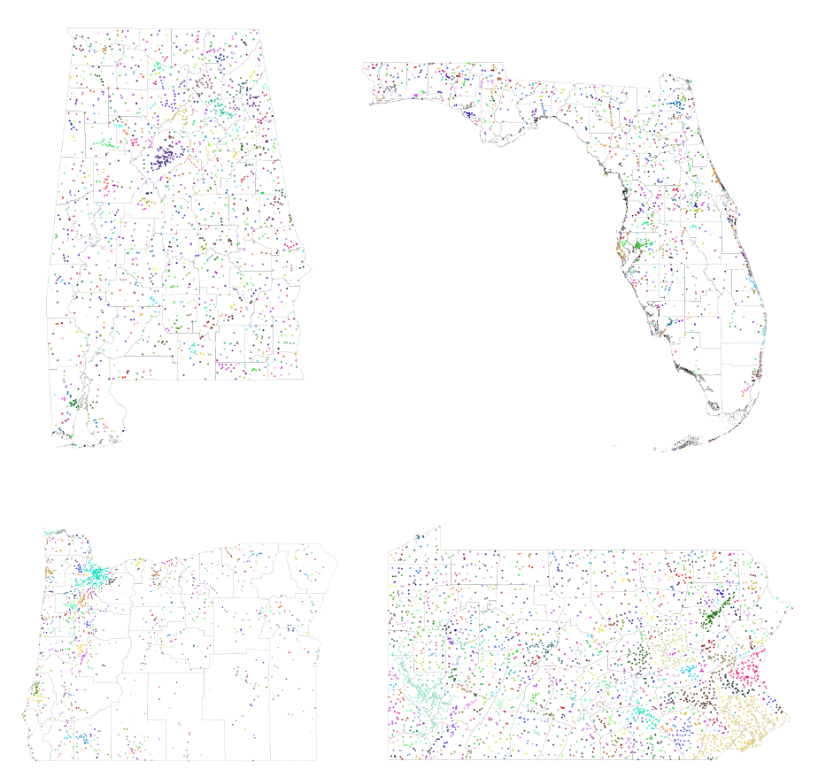
Figure 5: State-level maps of clustered places with county borders
Alabama Florida
Oregon Pennsylvania
Notes: is gure maps our geocoded places in four states: Alabama, Florida, Oregon, and Pennsylvania. We
highlight the county borders in each state to emphasize the granularity of our geocoded places relative to the
larger counties.
23
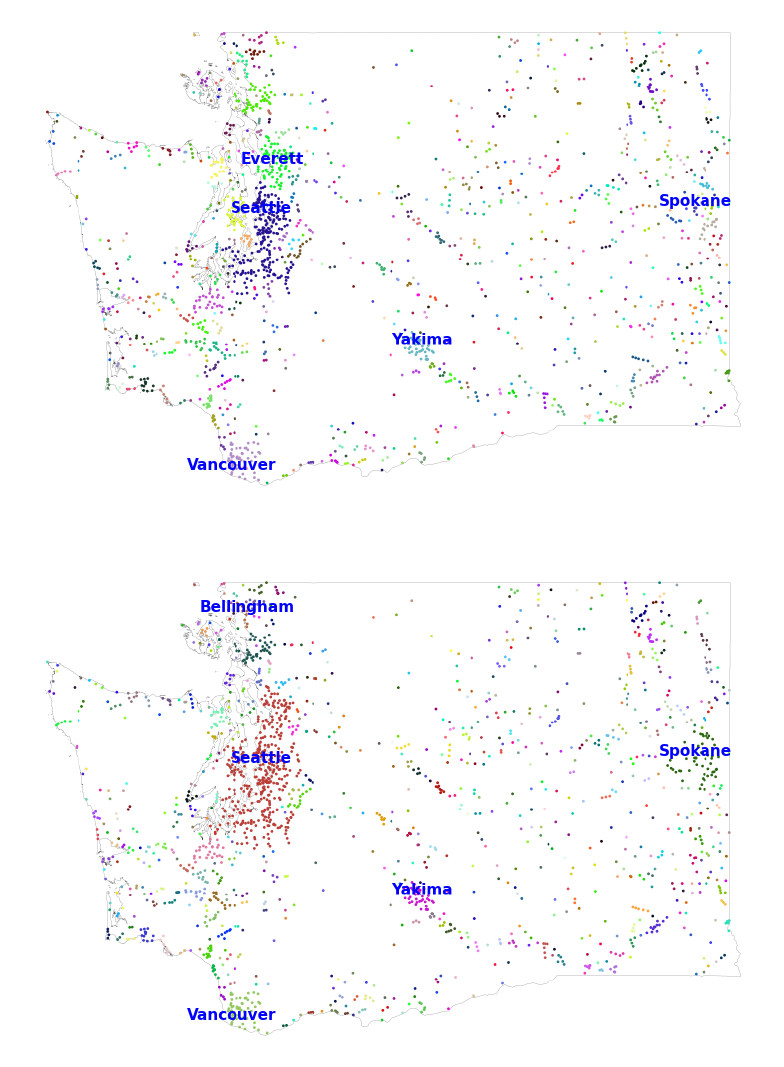
Figure 6: Clusters in Washington State with dierent levels of K
cluster
K
cluster
= 5
K
cluster
= 500
Notes: is gure maps our geocoded places in Washington with more conservative clustering (K
cluster
= 5) and
more aggressive clustering (K
cluster
= 500). e largest dierence is in the implied size of the Seale metropolitan
area.
24
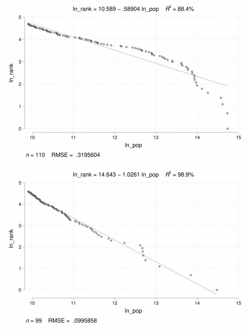
Figure 7: Zipf’s Law for 1870 places with population 20,000+ (CPP vs. IPUMS)
Notes: is gure plots log(population) vs. log(rank) for all cities with population greater than 20,000 in 1870
labeled by IPUMS (top panel) and in our geocoded places (boom panel).
25
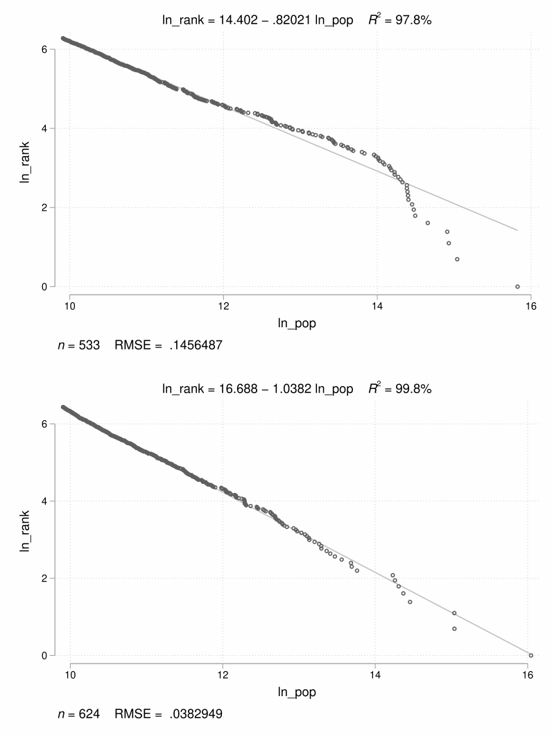
Figure 8: Zipf’s Law for 1940 places with population 20,000+ (IPUMS vs. CPP)
Notes: is gure plots log(population) vs. log(rank) for all cities with population greater than 20,000 in 1940
labeled by IPUMS (top panel) and in our geocoded places (boom panel).
26
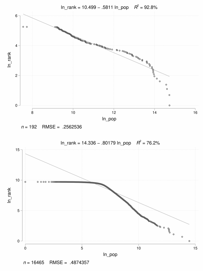
Figure 9: Zipf’s Law for all places in 1870 (IPUMS vs. CPP)
Notes: is gure plots log(population) vs. log(rank) for all cities in 1870 labeled by IPUMS (top panel) and in our
geocoded places (boom panel).
27
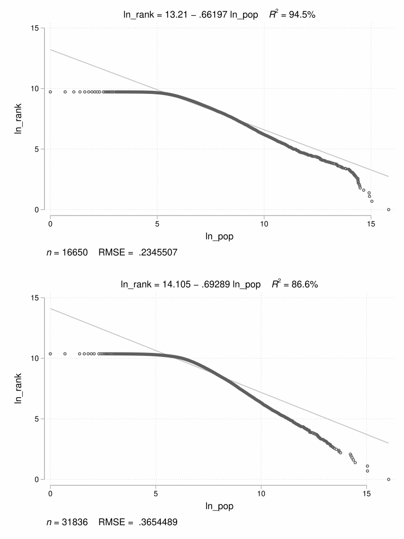
Figure 10: Zipf’s Law for all places in 1940 (IPUMS vs. CPP)
Notes: is gure plots log(population) vs. log(rank) for all cities in 1940 labeled by IPUMS (top panel) and in our
geocoded places (boom panel).
28
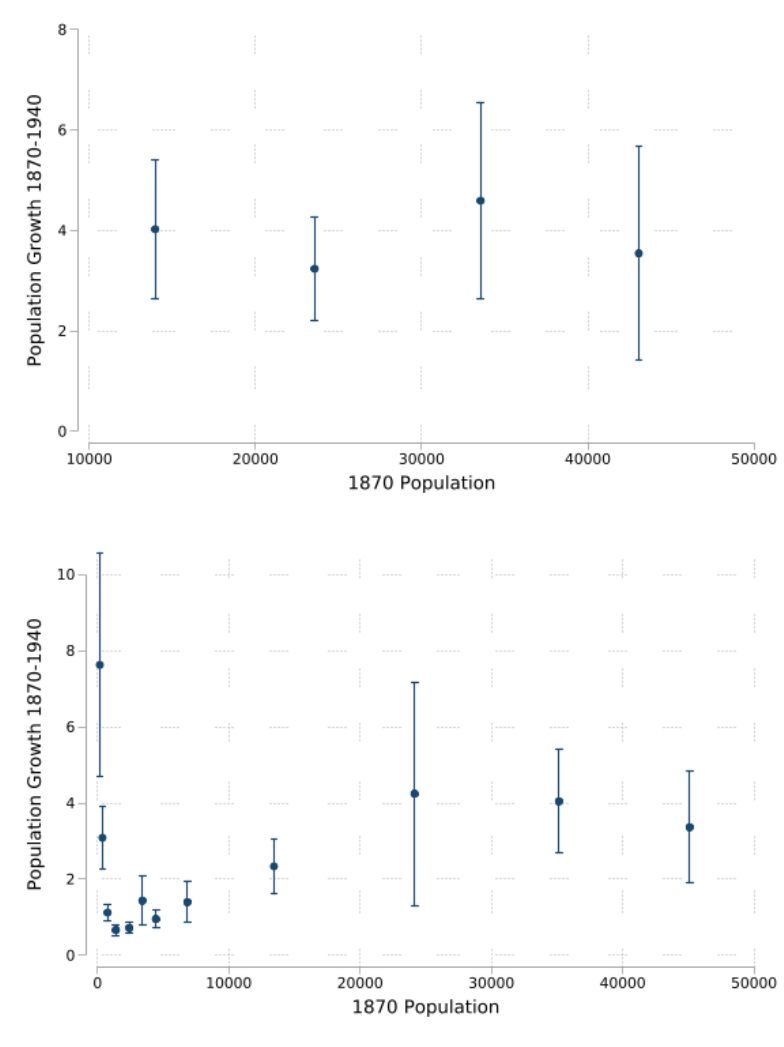
Figure 11: Gibrat’s Law (IPUMS vs. CPP)
Notes: is gure tests Gibrat’s Law by ploing the relationship between population growth rates between 1870
and 1940 (y-axis) and baseline 1870 population levels for places labeled by IPUMS (top panel) and in our geocoded
places (boom panel). We plot binscaered growth rates. We focus on places with population less than 50,000 to
emphasize the dierence between the two approaches for small cities and towns. e y-axis units is percent
growth, so a value of 2 indicates that a place tripled in size from 1870 to 1940.
29

A Data Appendix
is appendix describes that data and approach that we use to standardize place names in the
historical censuses.
• Place name variables in IPUMS data:
1. 1790–1820: township
2. 1830: general township orig
3. 1840: locality
4. 1850: stdcity, us1850c 0043, us1850c 0053, us1850c 0054, us1850 0042
5. 1860: us1860c 0040, us1860c 0042, us1860c 0036
6. 1870: us1870c 0040, us1870c 0042, us1870c 0043, us1870c 0044, us1870c 0035, us1870c 0036
7. 1880: mcdstr, us1880e 0071, us1880e 0069, us1880e 0072, us1880e 0070
8. 1890: stdcity, us1900m 0045, us1900m 0052
9. 1900: stdcity, us1900m 0045, us1900m 0052
10. 1910: stdcity, us1910m 0052, us1910m 0053, us1910m 0063
11. 1920: stdmcd, stdcity, us1920c 0057, us1920c 0058, us1920c 0068, us1920c 0069
12. 1930: stdmcd, stdcity
13. 1940: stdcity, us1940b 0073, us1940b 0074
• State variables in IPUMS data:
1. 1790–1820: fullstate (name)
2. 1830: self residence place state (name)
3. 1840: fullstate (name)
4. 1850: stateicp (code)
5. 1860–1870: statep (code)
6. 1880: stateicp (code)
7. 1900–1940: statep (code)
• County variables in IPUMS data:
1. 1790–1820: county (name)
2. 1830: self
residence place county (name)
3. 1840: county (name)
4. 1850: stcounty (code)
30
5. 1860–1870: countyicp (code)
6. 1880–1930: stcounty (code)
7. 1940: countyicp (code)
Location cleaning procedure:
• Substitute mt. (and mt followed by a space) with mount, and st. with saint. Note that we
cannot simply substitute st with saint because sometimes place names do end in st, but if
the string starts with st followed by a space then we substitute it with saint
• Substitute Indian reservation with reservation to match external sources of place names
• Remove anything in parentheses (e.g., (i), (ii), etc.)
• Remove numbers, commas, question marks, periods, parentheses, and slashes (/)
• Remove range(s) if the range is preceded and followed by a space or if it it’s at the end of
the string and preceded by a space
• Remove substrings that match any of the following (note the space at the end of some
strings): ’police jury’, ’justice ward’, ’court house’, ’militia district’, ’civil district’, ’justice
precinct’, ’election district’, ’undetermined’, ’not stated’, ’ village’, ’tract’, ’ ward’, ’assem-
bly district’, ’district’, ’no
˙
’, ’precinct’, ’subdivision’, ’beat’, ’plantation’, ’census designated
place’, ’post oce’, ’township of ’, ’town of ’, ’borough of ’, ’city of ’
• Remove ward or township followed by a space if it’s at the beginning of the string
• If the place name at this point contains “division” return an empty string (note that at this
point we’ve already taken care of subdivisions etc.)
• Remove “[east, west, south, north] side” or “[east, west, south, north]ern side” from the
string
• Substitute multiple spaces with only one
• If at this point the place name string has less than two characters or corresponds to town-
ship(s) or ward(s) return an empty string
• Trim white spaces
• Force all leers to lowercase
Extra Cleaning for Round 3:
• Drop hyphens (-)
• Drop cardinal points (south, north, east, west) and their adjectives (southern, northern,
eastern, western)
31
• Drop township and point when preceded by a space
• Remove all the spaces to standardize our merge process
Geotag procedure:
• Load GNIS data
• Load county shape le from NHGIS. We standardize IPUMS county variables to match 3-
digit FIPS variables per IPUMS documentation. IPUMS county variables are usually iden-
tical to FIPS standards. An exception is Maryland, where IPUMS county identiers are
shied relative to FIPS codes. We manually adjust these codes to match shapeles
• For all the decades at and aer 1900, we load the point place les downloaded from NHGIS.
We standardize the place names to match the format of our raw census place strings.
• We determine the order in which we consider the raw census place name variables by
ordering the variables from most unique places to least unique places within each year.
e reason for this is that the more unique names there are, the more disaggregated this
variable is likely to be. e more standardized the place name is, the fewer unique values
of places we see in the raw les (for example, Charlestown and Boston may be combined
into one place called Boston in some of the place name variables).
• We have lexicographic preferences over the sequence of census place names. In other
words, we have three matching rounds that we apply to the rst place name in our or-
dered list, if do not get a match we move to the second one, and so on.
• For decades at and aer 1900, we try to match our census place names to NHGIS and GNIS
places. ere are three matching rounds:
– Round 1: nd the place name in the NHGIS/GNIS places le that is most similar to the
one in the census microdata. We require that the potentially matching NHGIS/GNIS
place needs to be in the same state and county as the place name from the IPUMS
le (using historical boundaries) and also that the string matching score using the
FuzzyWuzzy package in Python is ≥ 95.
– Round 2: same thing as above with the slight dierence that the matching require-
ment is no longer a FuzzyWuzzy score ≥ 95 but a Levenshtein distance of 1. Since
this threshold does not depend on the length of the place name, it is a less stringent
requirement for shorter place names (but a stricter requirement for long ones). Note
that here if there are multiple cities with a Levenshtein distance of 1, then we skip
this step for that place.
– Round 3: e same as round 1, with the exception that we apply the extra cleaning
described above to the raw place names of cardinal references (e.g., strip Township,
cardinal points, etc.).
32
• We begin by aempting to nd census places in the NHGIS place point data, and we then
proceed to look in the GNIS le, where we consider the following feature classes in order:
populated place, locale, civil, census, area, beach, harbor, island, military, mine, park, post
oce, unknown, basin, bay, falls, rapids, reserve, reservoir, ridge, spring, stream, valley.
e classes are ordered in terms of importance. at is, we rst try to match the census
place names to cities in the GNIS feature class ‘populated place’, then we match the census
place names to locales, and so on.
• For each class of places in GNIS, we rst drop the “distant duplicates,” which we dene as
all the places that have the same exact name and are more than 5km apart, because we are
unsure which place to match to. Note that if two places have the same name and are within
5km, we keep the rst listed GNIS place.
• We look for matches in the NHGIS and GNIS features (in the order described above), rst
completing round 1 for NHGIS places, GNIS populated places, GNIS locales, GNIS civil
features,… until we match GNIS valleys. We then proceed to round 2, searching for NHGIS
places, then GNIS populated places,… We then proceed to round 3.
• We have an extra step for the GNIS data where we take all places with duplicates more
than 5km apart and we aempt to match our raw census place name to the GNIS duplicate
in the correct county. If there are multiple matches within the same county, we keep the
match with the lowest latitude.
• For 1850 data and all census years at or aer 1880, the census data contains enumeration
districts and we use them to impute the coordinates of towns that we are not able to geocode
in the previous steps. e procedure works as follows:
– if an as-of-yet ungeocoded place is in the same state, county, and enumeration dis-
trict as one (or more) place with known latitude and longitude, we assign the place
name the same longitude and latitude as the already geocoded place (if multiple places
within the same enumeration district have already been successfully geocoded, we use
the mean of the previously geocoded coordinates);
– if an as-of-yet ungeocoded place is in an enumeration district that is numerically
between two (non-necessarily adjacent) enumerations districts that contain already-
geocoded places and if the distance between these two enumeration districts is smaller
than 50km, then we assign to the ungeocoded place the mean of the means of the
already geocoded latitudes and longitudes of places in those enumeration districts.
Note that this corresponds to the midpoint between the two mean coordinates of the
geocoded enumeration districts. Note that we always use the average. For example, if
we have enumeration districts 1, 2, 3, 4 and we have geocoded coordinates for 1 and 4
that are within 50km of each other, then enumeration districts 2 and 3 would receive
the same coordinates, equal to the average of the coordinates of geocoded places in
enumeration districts 1 and 4.
33
• We then have a second round of matching where we take as-of-yet ungeocoded places and
search for them on Google Maps, taking the resulting longitude and latitude aer conrm-
ing that that Google-based longitude and latitude is in the correct historical county.
• We then have a penultimate round of matching that uses 1910 counties as our reference
geography to test whether cities fall within the right county boundaries. e Census data
seem to use some county or state names before they were ocial (e.g., West Virginia in
1860). For this reason, when comparing the coordinates that we obtain through our match-
ing procedure and the location on a contemporaneous map, we sometimes get false neg-
atives (i.e., towns that are outside a county although they should fall within). is step is
meant to x this problem by using a map with state and county boundaries that should be
somewhat stable.
• Lastly, we take all geocoded places and look for towns in a specic state that are unique in a
given year but geocoded in only some years and not others. is can happen, for example, if
the enumeration district imputation step nds a place that was otherwise missing in other
years. We take the longitude-latitude for that place in the geocoded year and assign it to
the ungeocoded place with the same name in other years.
34
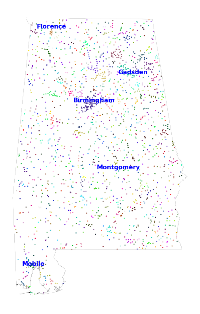
Figure A1: Alabama: Large map of clusters
Notes: is gure maps the geocoded places in Alabama, highlighting the ve largest clusters (with K
cluster
= 5)
35
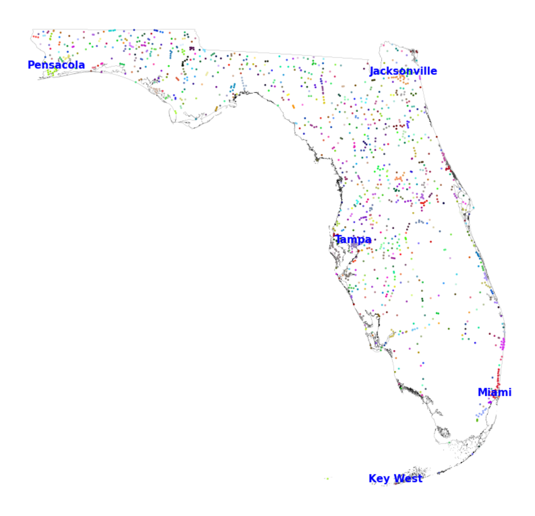
Figure A2: Florida: Large map of clusters
Notes: is gure maps the geocoded places in Florida, highlighting the ve largest clusters (with K
cluster
= 5)
36
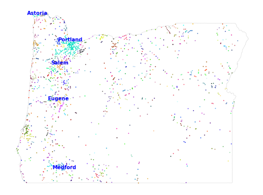
Figure A3: Oregon: Large map of clusters
Notes: is gure maps the geocoded places in Oregon, highlighting the ve largest clusters (with K
cluster
= 5)
37
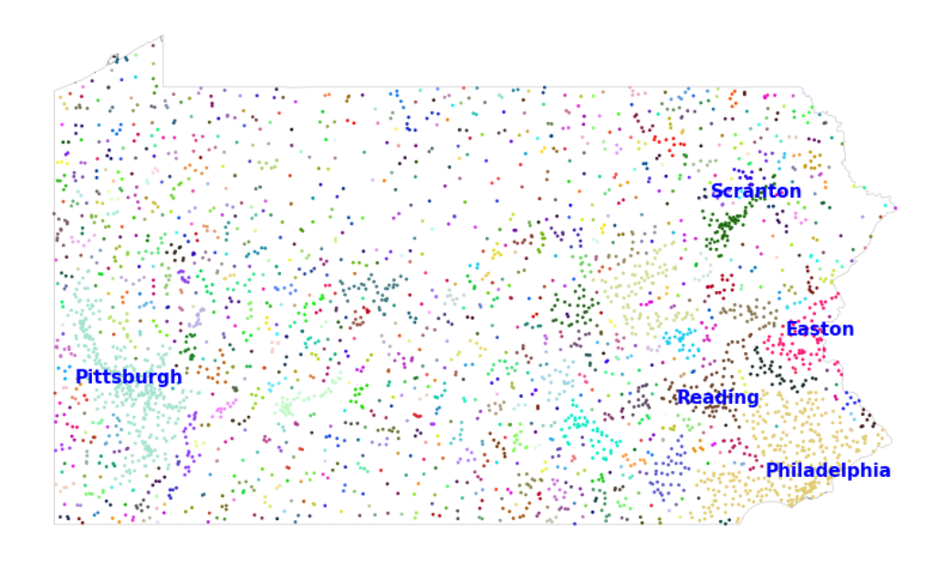
Figure A4: Pennsylvania: Large map of clusters
Notes: is gure maps the geocoded places in Pennsylvania, highlighting the ve largest clusters (with
K
cluster
= 5)
38
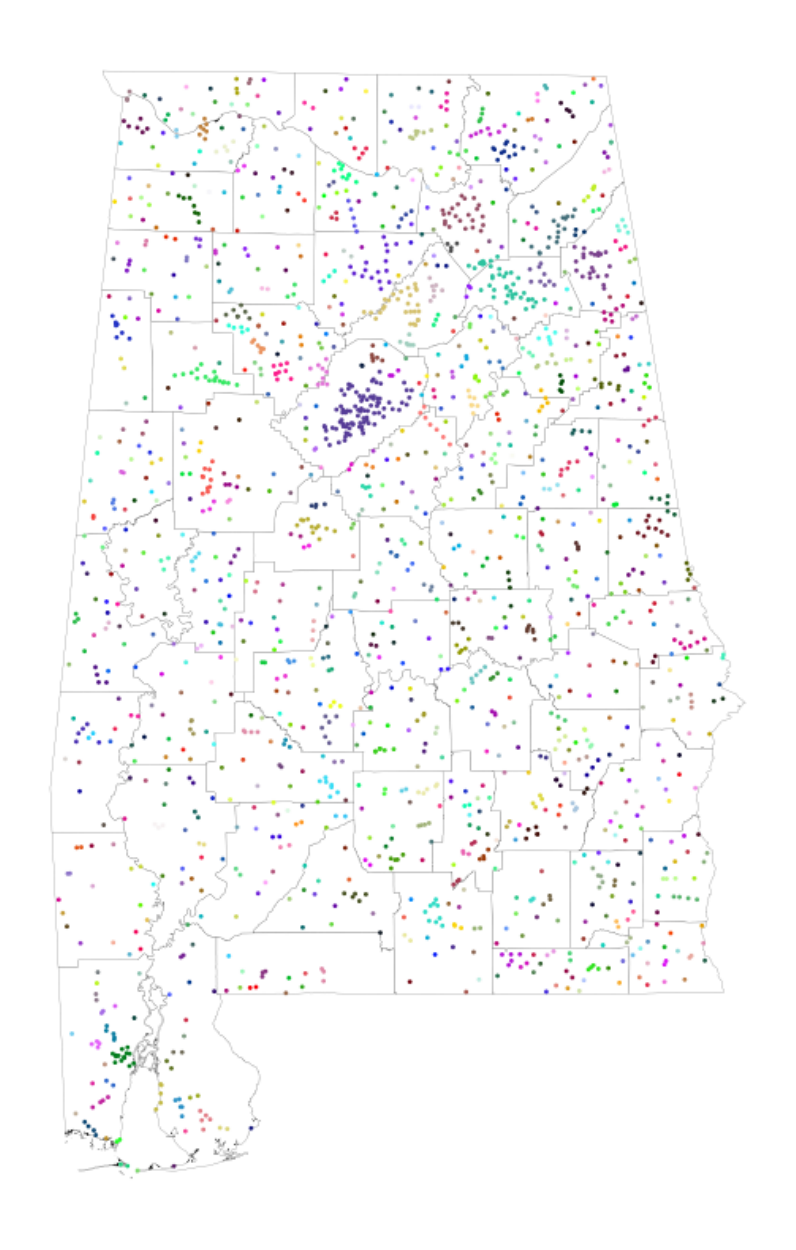
Figure A5: Alabama: Large map of clusters, with county borders
Notes: is gure maps the geocoded places in Alabama, highlighting the county borders in Alabama to emphasize
the large number of geocoded places in our data relative to the smaller number of counties. Sets of adjacent places
within the same cluster (K
cluster
= 5) are mapped with the same color.
39
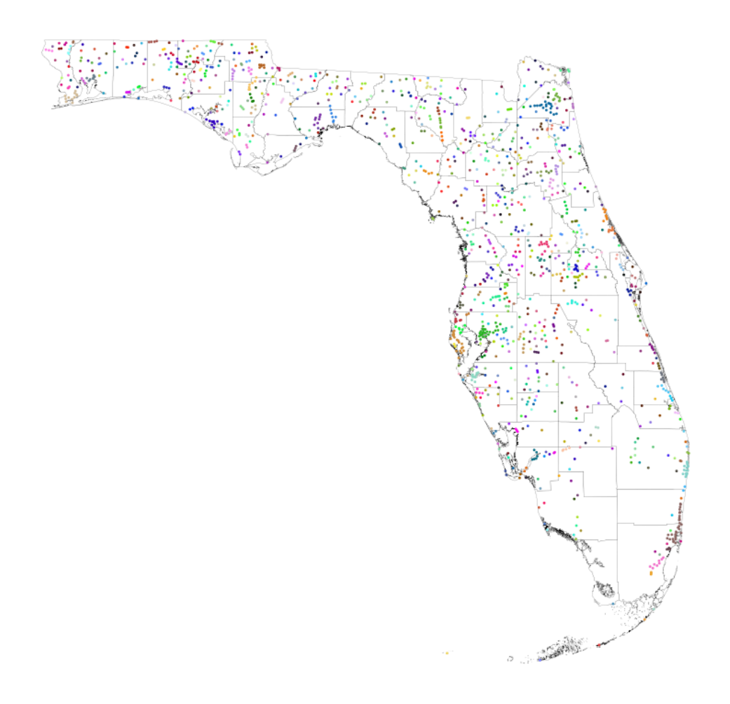
Figure A6: Florida: Large map of clusters, with county borders
Notes: is gure maps the geocoded places in Florida, highlighting the county borders in Florida to emphasize the
large number of geocoded places in our data relative to the smaller number of counties. Sets of adjacent places
within the same cluster (K
cluster
= 5) are mapped with the same color.
40
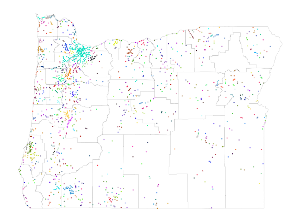
Figure A7: Oregon: Large map of clusters, with county borders
Notes: is gure maps the geocoded places in Oregon, highlighting the county borders in Oregon to emphasize
the large number of geocoded places in our data relative to the smaller number of counties. Sets of adjacent places
within the same cluster (K
cluster
= 5) are mapped with the same color.
41
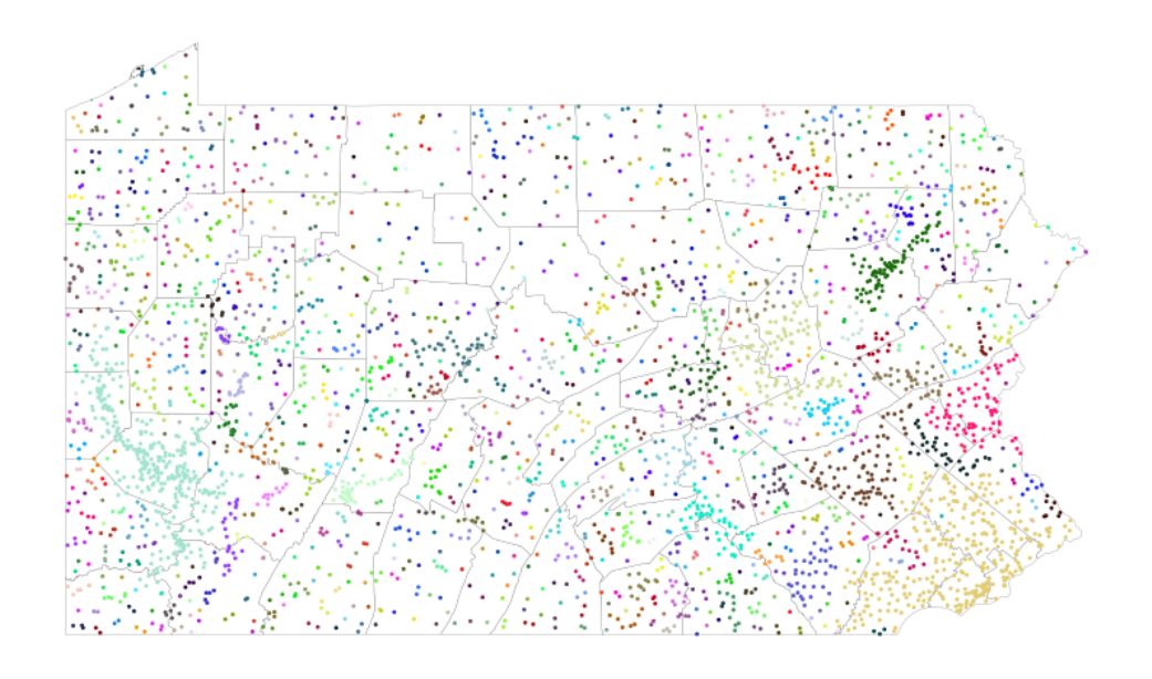
Figure A8: Pennsylvania: Large map of clusters, with county borders
Notes: is gure maps the geocoded places in Pennsylvania, highlighting the county borders in Pennsylvania to
emphasize the large number of geocoded places in our data relative to the smaller number of counties. Sets of
adjacent places within the same cluster (K
cluster
= 5) are mapped with the same color.
42
