
Using the Google Places
API and Google Trends
Data to Develop High
Frequency Indicators of
Economic Activity
by Paul Austin, Marco Marini, Alberto Sanchez, Chima Simpson-Bell, and
James Tebrake
WP/21/295
IMF Working Papers describe research in progress by the author(s) and are published to elicit
comments and to encourage debate.
The views expressed in IMF Working Papers are those of the author(s) and do not necessarily represent the
views of the IMF, its Executive Board, or IMF management.
2021
DEC

© 2021 International Monetary Fund
WP/21/295
IMF Working Paper
Statistics Department
Using the Google Places API and Google Trends Data to Develop High Frequency
Indicators of Economic Activity
Prepared by Paul Austin, Marco Marini, Alberto Sanchez, Chima Simpson-Bell, and James Tebrake
Authorized for distribution by J. R. Rosales
December 2021
IMF Working Papers describe research in progress by the author(s) and are published to elicit
comments and to encourage debate. The views expressed in IMF Working Papers are those of the
author(s) and do not necessarily represent the views of the IMF, its Executive Board, or IMF management.
ABSTRACT: As the pandemic heightened policymakers’ demand for more frequent and timely indicators to assess
economic activities, traditional data collection and compilation methods to produce official indicators are falling short—
triggering stronger interest in real time data to provide early signals of turning points in economic activity. In this paper, we
examine how data extracted from the Google Places API and Google Trends can be used to develop high frequency
indicators aligned to the statistical concepts, classifications, and definitions used in producing official measures. The
approach is illustrated by use of Google data-derived indicators that predict well the GDP trajectories of selected countries
during the early stage of COVID-19. To this end, we developed a methodological toolkit for national compilers interested in
using Google data to enhance the timeliness and frequency of economic indicators.
JEL Classification Numbers:
C81, E01.
Keywords: Reopening, COVID-19, High-Frequency Data, Business Register.
Author’s E-Mail Address:
3
Contents Page
I. MOTIVATION .......................................................................................................................................................5
II. SO URCE DATA....................................................................................................................................................7
A. Google Places and Google Trends .........................................................................................................7
III. METHODS ........................................................................................................................................................ 14
A. Operating Status Indicators.................................................................................................................. 14
B. Business Activity Indicators ................................................................................................................ 19
IV. USI NG GO OGLE DATA FO R GDP NOWCASTING .......................................................................... 26
V. CONCLUSIONS................................................................................................................................................. 29
REFERENCES......................................................................................................................................................... 47
Box
1. Textual Description of the Manufacture of Consumer Electronics Industry .....................22
Figures
1. Google Trend “Flights” - Canada...................................................................................12
2. Google Trends: Demand for Ford Escape - Canada ........................................................14
3. Operating Indicator (weighted by reviews) for Selected City Centers ..............................16
4. Business Re-opening Indicator for Selected City Centers................................................18
5. Review Activity Indicator .............................................................................................21
6. Change in Google Trends Compared to Change in Real Quarterly GDP ..........................25
7. Transportation and Storage: Comparison between Official Data (GDP-H), Google Trends
(TRE-H), and Reopening Indicator (REOP) for Selected Countries ....................................27
8. Transportation and Storage: Nowcasts for 2020-Q2 and 2020-Q3 ...................................29
Tables
1. Fields of Information that can be Extracted for Each Place using Google Places API.........9
2. Statistical Concept: Units ..............................................................................................10
3. Statistical Concept: Operating Status .............................................................................11
4. Statistical Concept: Territory .........................................................................................11
5. Statistical Concept: Size ................................................................................................12
6. Construction of Google Trends Index: Example .............................................................12
7. Search Topics Related to Consumer Electronics for Australia .........................................13
8. Construction of Operational Indicator-Example..............................................................15
9. Reopening Indicator ......................................................................................................17
10. Indicator of Business Activity Using Reviews ..............................................................19
11. Stock / Change in Reviews – Paris City Center Beauty Salons ......................................20
12. Monthly Google Trends SVIs at ISIC 4-digit level for Accommodation and Food Service
Activities (I) for Australia .................................................................................................23
13. Monthly Google Trends SVIs at ISIC Section Level for Accommodation and Food
Service Activities (I) for Australia .....................................................................................24
14. Transportation and Storage: Regression Results ...........................................................28
4
Annexes
I. Technical Aspects of Google Trends and Google Places API ..........................................31
II. Data and Methods with the Imfgoogle R Package ..........................................................41
5
I. MOTIVATION
To say the needs of users of economic statistics have changed since the start of the pandemic
would be an understatement. Things are simply not what they were. We have gone from a
world of short-term predictability to one where policymakers need to take a daily pulse of
economic activity and adjust course often. Data consumers have become accustomed to
seeing daily charts of health-related data. Case counts, moving averages and trends, cycles,
peaks, and troughs are now a common part of our vocabulary and daily conversations. Users
of economic data are now starting to demand a similar service from economic statisticians.
Tasked with identifying the path out of the pandemic—represented by letter shapes whether
that be V, W, U, K (choose your letter of choice)—data users and policy makers require
more frequent, timely and granular economic statistics.
The need to modernize is clear. Traditional economic data collection and processing methods
to produce indicators of economic activity do not meet the timeliness and frequency demands
of policymakers during a pandemic (or any other crisis for that matter). Even among those
countries with the most advanced statistical systems it often takes at least 45 to 60 days
following the reference period to get a reading on what is happening. As we have seen with
the pandemic, those 45 to 60 days can mean the difference between staying in business or
losing your business. Just over two-thirds of the 190 IMF member countries produce
quarterly estimates of gross domestic product (GDP). The rest produce annual measures of
GDP and most are released 9 to 12 months following the reference period. This means that in
many countries, statisticians will not have a final tally of the effect of the start of the
pandemic until sometime in late 2021 and those estimates will say very little about the path
of the economy since its onset.
Improving the timeliness and frequency of economic statistics while maintaining their quality
is a longstanding challenge in the realm of economic measurement. Economic statisticians
often refer to this as the timeliness versus quality tradeoff in which policy makers are told
they need to accept lower quality data if they want improved timeliness. When constrained
by traditional data sources and approaches used to compile economic indicators, this is
certainly the case. Economic statisticians need to examine new data sources and develop new
methods to provide users with the type of ‘statistical tickers’ they are becoming accustomed
to. As has been widely acknowledged, “big data” and the vast amount of data collected by an
increasing number of digital platforms can offer part of the solution. Statisticians need to
quickly figure out how to bridge the gap between “big data” and official measures of
economic activity. The challenges facing many statistical organizations are:(1) acquiring the
source data; (2) processing these data; and (3) integrating these data with high quality official
measures of economic activity to improve their timeliness and frequency. Data available
from the Google Places and Google Trends Platforms may provide part of the answer.

6
Interest in the use of real time, non-traditional data sources
1
to measure economic activities is
not new. Elvidge et al. (1997) identified a correlation between illuminated areas, electric
power consumption, and GDP at the country level. Since then, the rapid growth of new
sources of big data—enabled by internet-based technologies—has expanded the toolkit for
tapping real-time information at a more scalable and granular level. Within the last decade,
scanner data on purchases, credit card transaction records, and prices of various goods and
services scraped from the websites of online sellers have been increasingly mainstreamed in
the compilation programs of statistical agencies in advanced and emerging economies.
Abraham et. al (2019) documents the progress made toward the goal—and the challenges to
be overcome to realize the full potential—of using big data in the production of statistics.
Exploiting online platforms for tracking economic developments gained traction as the data
observations harvested became longer, more accessible, and stable. The use of Google-
sourced data to forecast private consumption was explored by Schmidt and Vosen (2011);
and was followed by academic research in similar directions by Choi and Varian (2012) on
predicting economic activity, and by Luca (2016) on the impact of Yelp-based consumer
reviews on the restaurant industry, among others. Jun, Yoo and Choi (2016) traces the ten
years of research using Google Trends since the company made this source of data available
in 2006. Noting that the availability of timely data is a long standing challenge for
policymaking and analysis for low-income developing countries, Narita and Yin (2018)
explored the use of Google Trends data to narrow such information gaps. Many organizations
have since developed timely leading indicators using Google data (Google Trends, Google
Mobility data, Google APIs) that track well official measures of economic activity. More
recently, the OECD Weekly Tracker of GDP growth (2020) attempts to fill the gap in real-
time high-frequency indicators of activity with a large country coverage.
These research strands and experimental estimates have shaped our understanding of current
(now-time) economic trends. Building on this work, over the last year, the IMF Statistics
Department (STA) has been working with Google data to determine how data extracted from
the Google Places and Google Trends platforms can be processed for use by data compilers
in developing higher frequency and timely measures of economic activity that can be used to
increase the timeliness and frequency of official measures.
This paper is organized as follows. Section II describes Google Places API and Google
Trends and how they can be accessed by national statistical organizations. Section III
explains how country compilers and researchers can process these data and develop high
frequency indicators that align with the concepts, classifications, definitions, and methods
used to produce official measures of economic activity. Section IV shows an application of
these indicators to nowcast quarterly GDP of selected countries during the onset of the
COVID-19 pandemic. Section V offers some concluding remarks and next steps from this
1
Non-traditional data are characterized by high volume, velocity, and variety, often generated by social media,
web-based activities, machine sensors, or financial, administrative or business operations (BIS, 2021).

7
work. Finally, the technical annex describes the characteristics of the Google data used in this
research and the R package developed by the authors to reproduce the results.
2
II. SOURCE DATA
A. Google Places and Google Trends
Over the last five to ten years there has been a large push within the economic statistical
community to take advantage of a growing (exponentially) set of “big data” to produce
official statistics. This new source of information has the potential to address a lot of the
unmet needs of users of economic statistics – specifically as it pertains to their demand for
more timely data, published with a higher frequency and with more granularity. While these
data hold promise to significantly increase the timeliness, frequency, and granularity of
official statistics there are often significant challenges that need to be addressed before they
can be leveraged in the production of official statistics. These challenges are related to access
/ terms of use, coverage, and concepts.
The first, and generally most time-consuming challenge, is securing access to the data.
Before a statistical organization can consider using a particular data source in the production
of official statistics it needs to ensure it will have regular access to the data over the medium
term. It also needs some assurance that the composition of the data (coverage, variables,
frequency) will be stable during that period. Finally, it needs to ensure that its proposed use
aligns with the terms of use as outlined by the data owner and that these terms of use will be
stable over the medium term.
The second challenge that statistical organizations often face is coverage. Often big data can
be very timely and granular but may only cover part of the population of interest. For
example, a statistical organization may obtain scanner data from major retailers. If a
significant share of purchases occurs at local markets, the scanner data, while useful, only
provides partial coverage. In other cases, statistical organizations may require long-time
series to establish relationships with existing official estimates. Often big data can have broad
coverage, be timely and available on a daily frequency, but the data may only be available for
the previous two to three years, limiting their usefulness (at least in the short term).
The third challenge that statistical organizations face is the potential conceptual
misalignment between the big data source and the target statistic being produced. Statistical
frameworks outline and provide definitions for concepts such as revenue, income,
expenditure, exports, production, value added, etc. Statistical organizations are tasked with
developing statistics that provide a numerical representation of these concepts. To do this
statistical organizations often design collection instruments in which they tailor the questions
2
The results presented in this work and the accompanying datasets are available through an R package
developed by the authors. The ‘imfgoogle’ package is available upon request. Please refer to Annex II for more
deta ils.

8
to align with the concept they are trying to measure. In the case of big data, statistical
organizations have no control over the “question.” It is therefore often the case that the
concepts that underpin “big data” do not align with the concepts that the economic
statistician is attempting to measure. In these cases, the economic statistician will need to
make assumptions, build models, or make “second best measures” to align the big data with
the concept being estimated.
The data that can be acquired from the Google Places and Google Trends platforms exhibit
very few of these shortcomings. As shown below, data obtained from the Google Places and
Google Trends platforms address the economic statisticians’ needs with respect to access,
coverage and conceptual alignment with official statistics.
Google Places and Google Trends - Access
Data from the Google Places platform can be obtained using the Google Places API. The
Google Places API
3
is a service offered by Google that allows users to obtain information
about “Places” via an HTTP request. The requests return a JSON or XML file that is easily
integrated into a database. Uses of this information must comply with the Places API Policies
and Google Maps Platform Terms of Service. The terms of use support research purposes
and permit the results of research to be shared. There are limitations with respect to the
volume of data that can be extracted, and fees may apply depending on the volume of the
request and use of the information. From the perspective of compilers of official statistics,
the existence of the API addresses one of the key hurdles that are often associated with the
use of Big Data – access. The Google Places API provides seamless and stable access to over
20 fields of information for each Place on the Google Maps Platform. In addition, the Google
Places API has policies which help reduce the risk of using these data in the compilation of
official statistics. For example, the Google Places API has a depreciation policy which they
provide users with at least one year’s notice if they intend to change or discontinue a field.
This provides ample lead time for statistical organizations to adjust processes and methods.
One challenge facing statistical organizations is the cost of access. For data to be useful,
statistical organizations require a significant amount of data. Given the scope of their data
needs, they are required to pay. During COVID-19, this limitation is being addressed by
Google. Google has launched an
initiative to support nonprofit organizations with COVID-19
response efforts to access its data, free of charge, provided the applications have a public
good element. Since production of official statistics generally fall within the public good
category, there is opportunity for statistical organizations to negotiate access free of charge.
Google Trends is a public website (trends.google.com) managed and maintained by Google
that facilitates analysis of Google search queries. There is no charge to use the website or
extract information from the website. The information can be downloaded into CSV files, the
charts can be captured as images, shared, or directly embedded into webpages. The terms of
3
https://developers.google.com/places/web-service/overview.
9
use are governed by Google’s Terms of Use and Privacy Policy. While Google does not
provide an API to access the Google Trends data several publicly available web-scraping
scripts have been developed that facilitate the extraction of data. From the perspective of
statistical organizations, the data are highly accessible and the use of these data in the
compilation of official statistics falls within the Terms of Use and Privacy Policy outlined by
Google. The methodology Google uses to produce the trends data are documented and
available on the Google Trends website.
Google Places and Google Trends - Coverage
Both Google Places and Google Trends have wide (near census) coverage. It is safe to
assume that in the countries where Google operates the Google Places platform contains a
near census of Places - everything from businesses, to places of interest, to government
offices. This is important since it implies that the estimates produced using these data will be
very representative of the population of interest. In addition, given that the Google Places
platform contains a near census of Places, scientific samples of this population can be drawn,
and the characteristics and activities of the sample can be inferred on the population.
Similarly, the Google Trends data contains broad country and topical coverage. In fact, given
the widescale use of the Google search engine, trends can be calculated for individual
businesses and products. From a coverage perspective, the data that can be obtained from the
Google Places and Google Trends platforms have enough coverage to be used by most
countries across most economic activities. Clearly, coverage is wide for countries where
Google is used as the primary Internet search engine and there is no restriction to its use.
Google Places – Conceptual Alignment
The Google Places API allows users to extract information about Places from the Google
Maps Platform. In total, users can extract 23 fields of information for each Place as identified
in Table 1.
Table 1. Fields of Information that can be Extracted for Each Place using
Google Places API
Basic Fields
4
Address Component
Address
Business Status
Formatted Address
Viewport
Location
Icon
Name
Photo
Place ID
Plus Code
Typ e
4
https://developers.google.com/places/web-service/place-data-fields.

10
URL
UTC Of f set
Vicinity
Contact Fields
Phone Number
International Phone Number
Opening Hours
Website
Atmosphere Fields
Price Level
Rating
Reviews
User Ratings Total
The usefulness of these data in the production of economic indicators is determined, in part,
by how well these fields align with the target concepts outlined in international statistical
standards such as the System of National Accounts, Balance of Payments Statistics and
International Standard of Industrial Classification (ISIC).
The statistical unit is one of the most important concepts underpinning the production of
official statistics. It represents “the entity about which information is sought”
5
and ultimately
for which statistics are produced. The Google Places statistical unit is the Places ID. The
Google Places platform defines a Place as a “business, landmark, park, and intersection.” It
reflects an entity with a physical presence, where activity takes place which has a specific
and identifiable location. In the field of economic statistics, there are two types of statistical
units – households and legal entities. Legal units are generally classified into sectors or
industries (activities). When classified to activities a statistical hierarchy is adopted. This
statistical hierarchy moves from an enterprise, to an establishment, to a kind of activity unit /
local unit.
6
In the statistical domain a local unit is defined as “an enterprise or a part of an
enterprise (for example, a workshop, factory, warehouse, office, mine or depot) which
engages in productive activity at or from one location.”
7
The Google Places concept of a
Place aligns well with the statistical concept of a local unit. Given Google also identifies the
“place type,” the combination of the Google Places location information with the Google
Places “place type” approaches the statistical concept of an establishment. The conceptual
alignment between the Google Places Place and the statistical concept of a local unit or
establishment can therefore be regarded as “High.”
Table 2. Statistical Concept: Units
Target Statistical
Concept
Google Field
Subjective degree of alignment with
statistical concepts.
Local Unit
Places ID
High
5
https://unstats.un.org/unsd/classifications/Econ/Download/In%20Text/ISIC_Rev_4_publication_English.pdf (p.15).
6
https://unstats.un.org/unsd/classifications/Econ/Download/In%20Text/ISIC_Rev_4_publication_English.pdf.
7
https://unstats.un.org/unsd/classifications/Econ/Download/In%20Text/ISIC_Rev_4_publication_English.pdf (p.17).

11
Establishment
Places ID / Places Ty p e
High
The business status indicator available on the Google Places Platform also aligns well with
the statistical concept of the operating status of a business. The Google Places business status
indicator identifies whether a business is “operational,” “temporarily closed” or
“permanently closed.” This status indicator aligns with the economic statistical concepts of
“births” and “deaths,” “entries” and “exits” or “capacity” that are employed by most
statistical organizations. In addition to being conceptually well aligned the business status
information available from the Google Places Platform is available in real-time and indicates
when a business is temporarily closed - something that is generally not available from
statistical registers.
Table 3. Statistical Concept: Operating Status
Target Statistical
Concept
Google Field
Subjective degree of alignment
with statistical concepts.
Business Status
Business Status Indicator
High
Most economic statistics are presented at some level of geographic detail, whether the data
are presented for a country as a whole or for a specific region(s). Economic statisticians often
employ the concept of a territory. A territory is generally reflective of a country’s geographic
boundaries with a few exceptions such as the land area associated with embassies or
consulates. Given the Google Places Platform provides access to the longitude, latitude and
address associated with each Place the Google Places data can easily be reconciled to the
statistical concept of a territory.
Table 4. Statistical Concept: Territory
Target Statistical
Concept
Google Field
Subjective degree of alignment with
statistical concepts.
Territory
Longitude / Latitude
High
Territory
Address
High
In addition to concepts such as territory and activity most economic statisticians require
information about an entity’s size. In most cases countries rely on business surveys or
administrative sources (such as taxation records) to obtain information about the size (e.g.,
revenue, number of employees) of an entity. While the Google Places Platform does not
contain information related to the revenue or employment of a Place, it does collect and store
what Google refers to as “Atmosphere Data Fields.” These fields include the number of
reviews associated with a given entity, its price level as well as the rating (scaled 1-5)
provided by reviewers. It is fair to assume that larger / more popular / successful places will
have more reviews. It is also fair to assume (but to a lesser degree) that a place with twice as
many reviews as another place is roughly twice its size (or at least twice as popular). Using
these assumptions, the number of reviews could therefore be used to proxy the size of a
Place. Information about the size of an entity will assist with statistical methods such as
sampling, weighting, and aggregation.
12
Table 5. Statistical Concept: Size
Target Statistical
Concept
Google Field
Subjective degree of alignment with
statistical concepts.
Size
Reviews
Medium
Size
Rating
Low
Size
Price Level
Low
Google Trends – conceptual alignment
Google Trends are a measure of interest in a topic relative to all other topics over time. A
topic can be anything from a person or event to a business or specific product. To the extent
that the topics relate to a business, industry, or product the trend could be indicative, at least
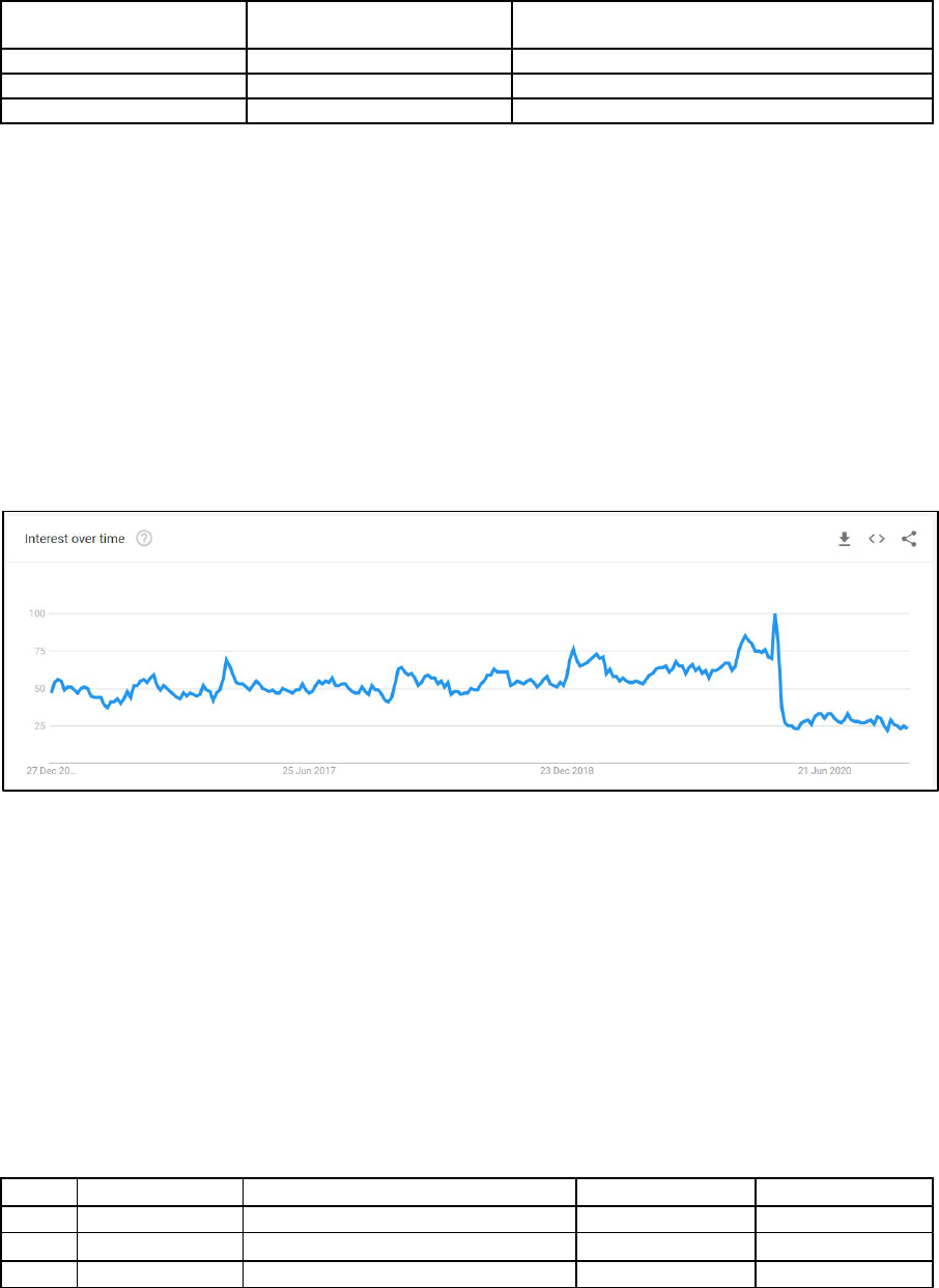
to some extent, of economic activity. For example, consider Figure 1 which shows the
Google Trend for the term “Flights” for Canada. The “interest” in flights in Canada declined
significantly towards the end of the first quarter of 2020 due to the COVID-19 travel
restrictions imposed by the Canadian Government. This is indicative of the decline in
economic activity that occurred in the Canadian Air Transportation Industry during this
period.
Figure 1. Google Trend “Flights” - Canada
Source: Google Trends – July 2020.
To illustrate how a “Google Trend” is calculated consider the following example. Assume
there are 10,000 searches in week 1 in a region and that 1,000 are related to restaurants. The
level of interest in restaurants is therefore 1,000/10,000=.1. Assume that each week we
measure the level of interest in restaurants (e.g., week 2=.08, week 3=.09) as illustrated in
Table 6. The weekly level of interest in restaurants is indexed to the week with the highest
level of interest (week 4 in our example). Using search activity as a proxy for demand for
restaurant services the trend would be interpreted as an indication that demand for restaurant
services was increasing in the first four weeks, stable over the next three weeks and declining
in the final weeks. This provides valuable information about turning points in activity.
Table 6. Construction of Google Trends Index: Example
Week
Total Searches
“Restaurant” Searches
Search Intensity
Trends Index
1
10000
1000
.1
83
2
10000
800
.08
67
3
10000
900
.09
75

13
Week
Total Searches
“Restaurant” Searches
Search Intensity
Trends Index
4
10000
1200
.12
100
5
15000
1200
.8
67
6
12500
1000
.8
67
7
10000
800
.8
67
8
10000
700
.7
58
9
10000
600
.6
50
10
10000
500
.5
42
The amount of information available via this platform is extensive. The platform provides
users with near worldwide geographic coverage and could be considered universal coverage
of social, economic, and environmental topics. This detail is an advantage and a
disadvantage. Given the almost infinite number of topics, the key challenge is selecting those
topics that are most indicative of a given economic activity. Therefore, it is necessary to
either group topics together into meaningful categories or select a sample of topics that
correspond to the activity of interest. With respect to the former, Google has developed an
algorithm to aggregate search topics into 1000+ “trend” categories. Google identifies the
most popular search topics related to category and aggregates the data by category. This
aggregation can be done by region and for different periods of time. For example, the
category “Consumer Electronics” for Australia is an aggregation of search topics in Table 7.
Table 7. Search Topics Related to Consumer Electronics for Australia
Source: Google Trends – July 2020.
In addition to obtaining trends by category it is also possible to extract trends for specific
businesses/products. For larger firms there are enough searches made that allow trends to be
calculated. For example, trends are available for Sandals Resorts, Cineplex Entertainment,
The Home Depot, Ikea Furniture Company, Holiday Inn Hotels, Oh Henry! Chocolate bar,
Ford Escape (see Figure 2), and Xbox Console in various countries. Assuming at company /
product level, there is a relationship between searches and business activity, having this
detail improves the potential of using Google Trends as an indicator of economic activity.
Radar
Apple Ultra-high-definition television
Bureau of Meteorology Television Kmart Pharmacy
The Good Guys Canon Kmart
Xbox Canon Rain
Xbox One JB Hi-Fi
Meaning
Camera Apple Weather radar
Headphones
Battery charger Soundbar
Australia Sony Bunnings Warehouse
Xbox Price
Fitbit
PlayStation 4 Fortnite Smart TV
Loudspeaker PlayStation 4 Pro JBL
Television set Microsoft Xbox One X Watch
Garmin Ltd.
Nintendo Switch Nintendo
Samsung Electronics New South Wales Education Standards Authority Netflix
Samsung AirPods Garmin Forerunner 235
Samsung Group Oppo reddit
4K resolution Reddit
Related Topics
14
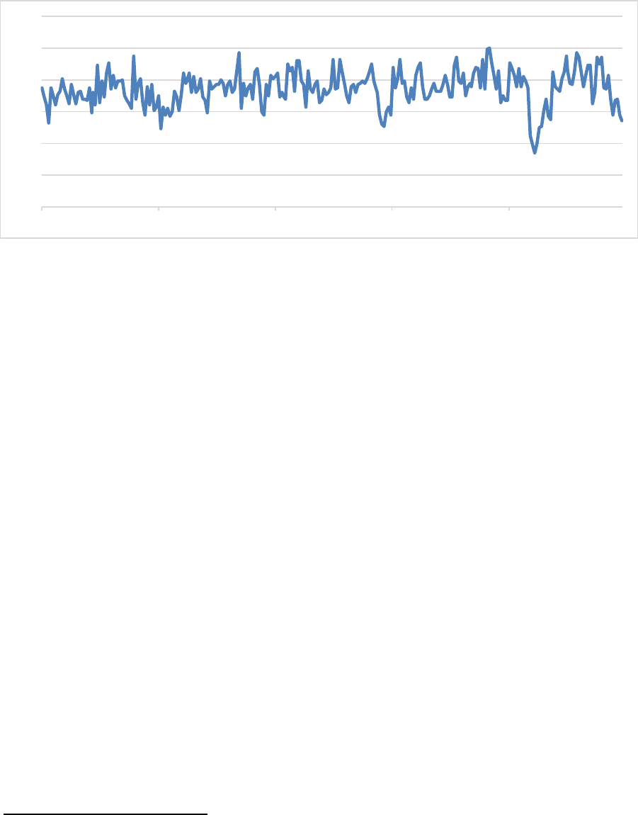
Figure 2. Google Trends: Demand for Ford Escape - Canada
Both the Google Places and Google Trends platform are a rich data source that align well
with the type of data sources used to compile official statistics. Data acquired from the
Google Maps platform closely aligns with the type of data used by national statistical
organizations in the production of business status and dynamic type statistics. These data
may be of use in helping better understand the business population and some of the entry and
exit dynamics at a very granular geographic level of detail. The Google Trends data, when
properly filtered, could highlight sudden turning points, and be used to improve the
timeliness and frequency of official measures. The next section of this paper outlines how the
Google Places and Google Trends data described above can be processed and transformed
into a set of economic indicators consistent with the classifications and concepts of official
measures.
III.
METHODS
A. Operating Status Indicators
The Google Places API permits users to extract the operating status of each place identified
on the Google Places platform. Places are given the status of “Open,” “Temporarily Closed”
or “Permanently Closed.” This information can be used to produce several useful business
dynamic indicators. If we assume that the Google Places Platform has a near census coverage
of all Places operating in a region and that the number of reviews is a good indication of the
relative size of one Place to another – we can use this information to measure the operating
status of Places in each geographic area.
8
Since there is a strong relationship between the
business’ operating status and its revenue and employment, these indicators could be useful
8
This a ssum ption is pa rticularly valid for consumer-facing establishments, such as stores and restaurants. For
businesses that do not sell directly to consumers, the number of reviews may not be a good indication of their
size. Statistics agencies can use existing business register or business survey data to a djust the rela tive weights
from reviews in a composite high-frequency indicator.
0
20
40
60
80
100
120
1/10/2016 1/10/2017 1/10/2018 1/10/2019 1/10/20 20

15
in providing an early signal of trends in the labor market or trends in aggregate economic
activity for the region.
Operational Indicator
The Google Places business status field can be used to construct an operational indicator. The
operational index represents the share of Places in each geographic region that are
operational at a given point in time weighted by the number of reviews. Weighting by
reviews is intended to capture the impact of the size of the business, in which businesses with
more reviews will have a larger impact on the movement in the indicator. To illustrate,
consider the following example (Table 8) in which the status of a sample of Places with
Place Type = “restaurants” f or a specific geographic region are tracked over a five-week
period. Since the Google Places API does not permit users to extract a census of all Places in
each geographic region, each week’s extraction is treated as a random and representative
sample of places for the region. Assume that these places are restaurants operating in the
same geographic area. In week 1, we note that Place A has 1000 reviews, Place B has 500
reviews, Place C has 500 reviews, Place D has 100 reviews, Place E has 400 reviews, and it
is temporarily closed.
The initial operational status of the business population of restaurants for this region is 84,
which simply represents the share of reviews of Places in operation. To understand the
dynamics of the indicator, the above example is extended such that:
• In week 2, establishment F is temporarily closed
• In week 3, establishment F re-opens
• In week 4, all establishments remain operational
• In week 5, establishment C permanently closes
Each week a business operational indicator can be calculated, as shown below.
Table 8. Construction of Operational Indicator-Example
Week 1 – Initial Status: Places A, B, C, and D operational
Business
Reviews
Share of Reviews
Business Status
Operational Indicator
A
1000
40
Operational
B
500
20
Operational
C
500
20
Operational
D
100
4
Operational
E
400
16
Temporarily Closed
2500
100
84
Week 2 – Place F is temporarily closed
Business
Reviews
Share of Reviews
Business Status
Operational Indicator
F
1000
37
Temporarily Closed
G
700
26
Operational
H
500
19
Operational
I
100
4
Operational
J
400
14
Operational
16
2700
100
63
Week 3 – All places are operational
Business
Reviews
Share of Reviews
Business Status
Operational Indicator
F
1000
33
Operational
K
700
24
Operational
L
500
17
Operational
M
400
13
Operational
J
400
13
Operational
3000
100
100
Week 4 – all Places are operational
Business
Reviews
Share of Reviews
Business Status
Operational Indicator
A
1100
30
Operational
B
900
25
Operational
C
600
17
Operational
M
500
14
Operational
L
500
14
Operational
3600
100
100
Week 5 – Place L permanently closes
Business
Reviews
Share of Reviews
Business Status
Weighted Population
A
1200
31
Operational
K
900
24
Operational
L
600
15
Closed Permanently
P
600
15
Operational
Q
600
15
Operational
3900
100
75
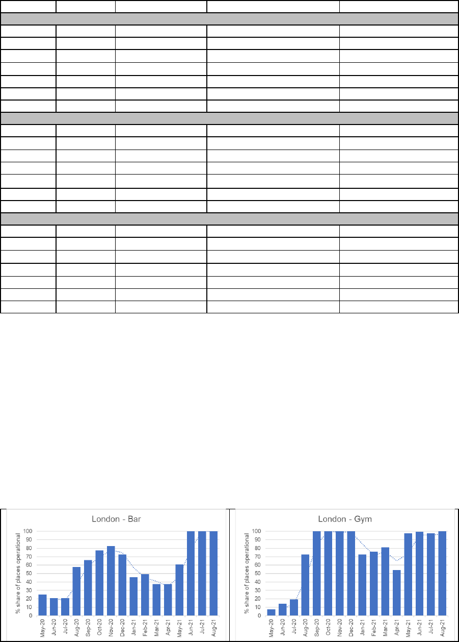
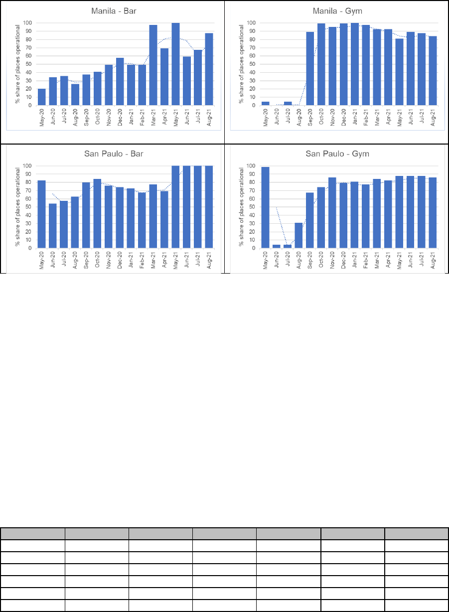
The above methodology was used to construct an operational indicator for several major city
centers for the period April 24, 2020 (the baseline) to August 10, 2021. The results indicate
that weighting by reviews has a significant impact on the index – introducing greater
variability. There is variation by city center and the operational status aligns well with the
timing of the various waves of the COVID-19 pandemic experienced by each of the city
centers. The variation by type of place is also consistent with the scope of the lockdown in
city centers where essential businesses remained open and non-essential business were
temporarily closed or altered their operations (e.g., curb-side pickup, limited capacity, limited
hours of operation). The following series of charts in Figure 3 compares bars with gyms for a
select set of city centers.
Figure 3. Operating Indicator (weighted by reviews) for Selected City Centers
17
Figure 3. Operating Indicator (weighted by reviews) for Selected City Centers
(continued)
Source: Goo gle Places API – Data Extracted between April 24, 2020 and August 10, 2021.
Business Re-opening Indicator
A second business status indicator that was constructed was a re-opening indicator. This
indicator is used to track the path and pace at which businesses that are temporarily closed in
a region re-open. This type of indicator was of particular interest during the COVID-19
pandemic where businesses were forced to shut down due to government regulations. This
indicator starts with the selection of a baseline cohort of places. In this case the cohort
consists of those firms that are temporarily closed. Each week (or selected time interval) the
status of each of these Places is examined to see if they have opened of if they remain
temporarily closed. The indicator reflects the share of businesses that were temporarily
closed in the baseline period that are now open. To illustrate consider the case of five firms
that were temporarily closed at the at time Baseline (Period B). Table 9 shows their status
(1=open, 2=temporality closed) in each of the following five time periods. The indicator is
calculated as the number of open firms divided by the total number of firms that were
temporarily closed in the baseline period.
Table 9. Reopening Indicator
Place
Period B
Period 1
Period 2
Period 3
Period 4
Period 5
A
2
2
2
2
2
2
B
2
2
2
2
2
1
C
2
2
1
2
1
1
D
2
2
1
1
1
1
E
2
1
1
1
1
1
Indicator
100
20
60
40
60
80
18
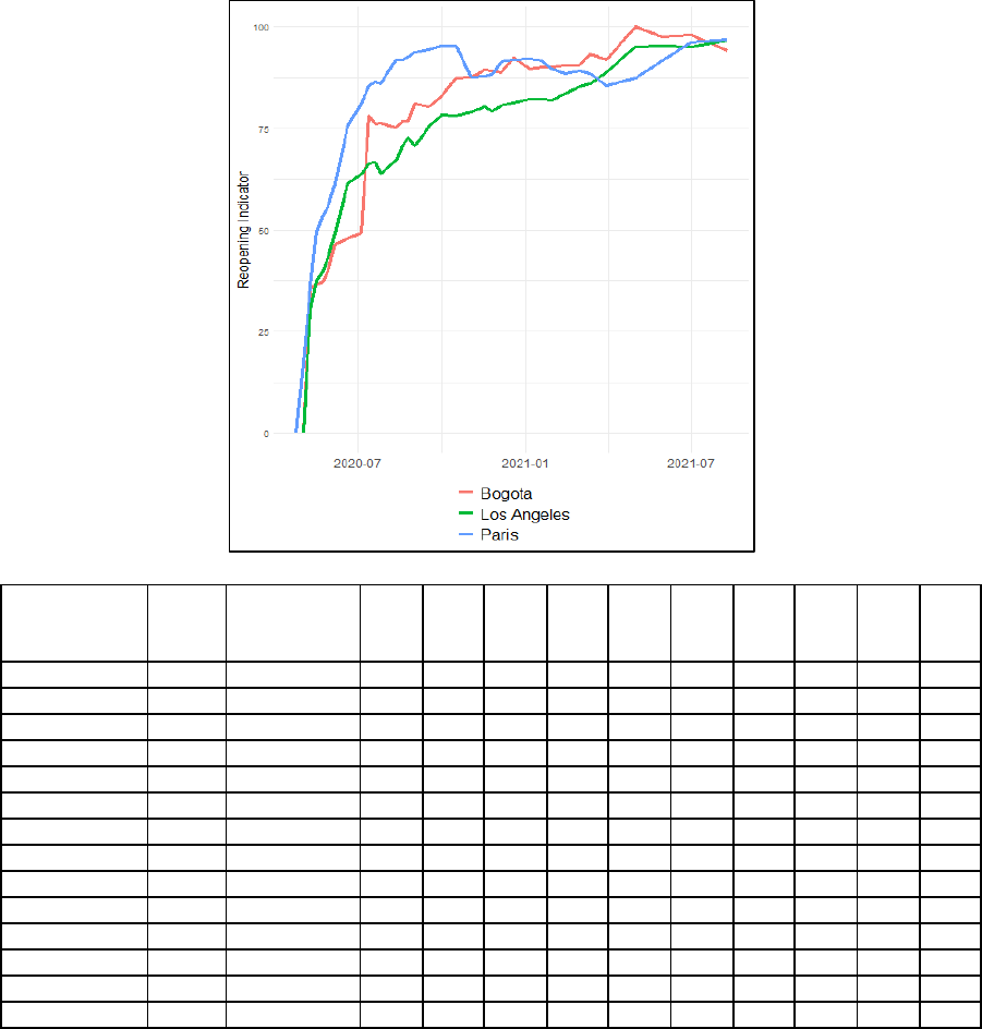
The above methodology was used to construct a business re-opening indicator for several
major city centers for April 24, 2020 (the baseline, where 0 percent of sampled businesses
had re-opened. Note below how some cities have a different baseline) to August 10, 2021.
The results are consistent with what is generally understood regarding the way different
governments implemented and lifted lockdown restrictions over the course of the pandemic.
Some governments imposed longer lockdowns in the hope that all businesses would be able
to move quickly to 100 percent operations after the lockdown. Other governments decided to
impose short lockdowns and leave the business to decide if it was economically beneficial to
open. Figure 4 illustrates the different path to re-opening taken in selected city centers.
Figure 4. Business Re-opening Indicator for Selected City Centers
city
sam
ple
size
baseline
24-
Apr
-20
24-
May
-20
26-
Jul-
20
26-
Aug
-20
3-
Nov
-20
30-
Jan
-21
31-
Mar
-21
1-
May
-21
1-
Jul-
21
10-
Aug
-21
Atlanta
503
2-May-20
59
82.9
96
97
96.8
97.6
98.6
98.8
99
Bogota
339
2-May-20
37.2
76.4
76.7
87.6
90
92
100
97.9
94.1
Casablanca
209
17-May-20
9.1
32.5
40.7
47.4
54.5
60.3
93.8
65.1
67.9
Istanbul
566
24-Apr-20
0
41.7
64.7
78.3
83.6
83.9
88.5
94.9
88.7
91.5
Lagos
180
24-Apr-20
0
25
38.3
38.9
53.9
58.3
62.8
98.3
76.7
76.1
London
842
24-Apr-20
0
53.4
84.8
93.1
97.1
80.8
79
89.7
97.9
98.5
Los Angeles
1,001
2-May-20
40
64
72.8
79.1
82
88.8
95
95
96.6
Madrid
1,437
24-Apr-20
0
44.6
75.9
87.3
92.3
92.9
94.7
98.3
95.8
95.9
Manila
2,750
24-Apr-20
0
41
70.1
79.6
84.6
88.1
89.8
96.6
92.1
92.8
Milan
936
24-May-20
0
59.1
77.1
84
81.9
86.3
95.8
92
90.5
Mumbai
2,939
24-Apr-20
0
45.6
66
72.8
85.7
92.8
94.2
97.2
93.4
93.9
New York
1,278
24-Apr-20
0
47.4
75.7
84.7
92.4
92.3
94.3
96.9
97.2
97
Paris
1,645
24-Apr-20
0
53.5
86
92.5
87.7
89.7
85.6
87.4
96.2
96.9
Rome
1,343
17-May-20
25.4
64.6
82.7
88.2
88.3
89.4
97.2
93.8
94.6

19
Sao Paulo
526
24-Apr-20
0
35.6
64.4
66.5
79.7
84.6
81.2
93
89.7
89.4
Sydney
359
2-May-20
47.4
84.7
86.9
91.6
94.4
95.8
97.2
76
74.9
Tel Aviv-
Yaf o
1,045
17-May-20
16.2
62.3
70.8
76.3
77.1
85.4
98.7
94.6
87.4
Tokyo
416
24-Apr-20
0
51.2
95
94.7
96.6
96.4
96.4
88
97.6
97.8
Toronto
978
24-Apr-20
0
42.1
90.8
93.4
94.7
84.6
89.9
87.1
88.9
95.9
Source: Google Places API – Data extracted fro m April 2020 to August 2021.
B. Business Activity Indicators
While the above indicators are intended to capture the evolution of the operation status of the
Places population, they do not fully capture the economic activity of the Places. To do this,
we require some indication of activity. As noted earlier, Google Trends capture the interest in
a topic relative to all other topics at a given point in time. If we assume that there is a
relationship between changes in interest in a topic(s) and changes in business activity the
Google Trends could be used as a proxy for business activity (at least in the short term).
Similarly, the Google Places API permits users to extract reviews from the Google Places
platform. These reviews are generally posted following some form of engagement with the
Place. If we assume that reviews reflect engagement, then this information can also be used
as a proxy for business activity. In the world of official statistics, business activities are
aggregated and classified in a systematic way. Most countries use the ISIC Rev. 4 (or some
variant of it) to classify business activities. It therefore seems appropriate that if we want to
use the Google Trends and Google Reviews data to proxy business activity we first need to
aggregate and classify these indicators by the ISIC Rev. 4.
Google Reviews as an Indicator of Business Activity
The Google Places API permits users to extract the number of reviews posted for a given
Place. In addition to the review the API also allows users to extract the average rating
provided for a Place. Ratings range from 1 (poor) to 5 (excellent). It is assumed higher
change in ratings are correlated with higher economic activity. For this indicator, the rating
was used to adjust the number of reviews such that a Place with 100 poorly rated reviews
would have a lower weight than a Place with 100 highly rated reviews. Since the maximum
score for a review is 5 the “adjusted” number of reviews was calculated as (average rate / 5)
*(number of reviews). To illustrate consider the following Places, each with 100 reviews and
various average ratings:
Table 10. Indicator of Business Activity Using Reviews
Place
Reviews
Rating
Weighted Rating
Adjusted Reviews
A
100
1
.2
20
B
100
3
.6
60
C
100
5
1
100
The review information available from the Google Places API represents the accumulated
number of reviews at a point in time. In this sense they should be treated as a “stock” type
variable. Since we are interested in measuring the change in activity from one period to

20
another, the variable of interest is not the stock of reviews but the change in the stock of
reviews from one period to the next. In addition to focusing on the change in reviews we also
need to consider that the Places selected for a given period represent a sample of Places for
the given geographic region. Ideally, we would like to track the change in reviews for the
same set of Places over time to reduce any potential sampling errors in the estimate. To
address this issue a month-to-month matched sample approach is taken. The match sample
approach involves identifying an overlapping set of Places in two consecutive periods and
calculating the stock of reviews for each period for this set of Places.
9
The stock of reviews
for each period is then linked together to form a continuous time-series using the baseline
stock of reviews as the initial level. To illustrate, five samples of Beauty Salon Places in
Paris were selected for the months April, May, June, July, and August 2020. The linked
stock of reviews and the change in reviews is presented in table 11.
Table 11. Stock / Change in Reviews – Paris City Center Beauty Salons
Matched Sample
Apr-20
May-20
Jun-20
Jul-20
Aug-20
April-May
1,289
1,306
May-June
1,694
1,744
June-July
1,772
1,821
July-August
1,664
1,727
Linked Stock of Reviews
1,289
1,306
1,344
1,381
1,433
Change in Reviews
17
38
37
52
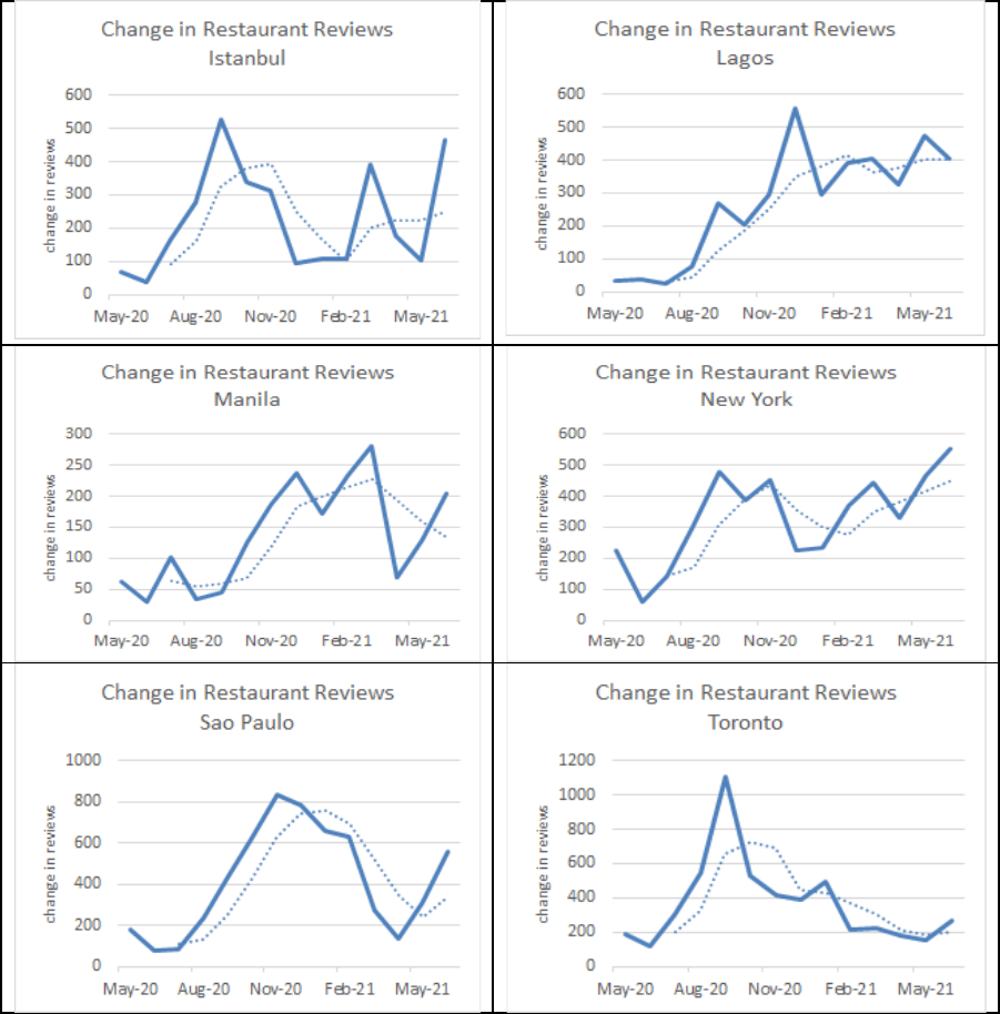
This methodology was applied to the monthly sample of Places collected in this project since
April 2020. The results align with the trends in activity over the last year in which activity
slowed during periods of lockdown or partial lockdown. The results also indicate that the
slowdown was the most pronounced during the first wave of COVID-19 and less pronounced
during subsequent waves – even though the subsequent waves were more pronounced in
terms of cases and severity of illness. The following series of charts in Figure 5 shows the
review activity for restaurants in Toronto, London, Manila, Johannesburg, Nairobi, Seoul,
and Sydney (the dotted lines in the figure are three-month moving averages).
9
The reason the same set of Places are not used for each month is because the sample size would deteriorate and reduce the
robustness of the estimate.
21
Figure 5. Review Activity Indicator
Source: Goo gle Places API – Data extracted from April 2020 to June 2021.
Google Trends as an indicator of activity
While there appears to be some conceptual and statistical relationship between reviews and
economic activity there are limitations associated with using reviews. First, up to this point, it
is not possible to construct a long time series of reviews due to unavailability of historical
Places data. Second, processes and extraction routines need to be set up at regular intervals as
not to introduce any bias into the estimates. Finally, the data are essentially self-reported, and
a key assumption is that the average reviews per visitor is constant over time. Given these
limitations and assumptions, additional activity indicators are required. As noted in Section
II, Google also provides access to information related to Google searches via the Google
22
Trends website. The challenge with using Google Trends data is how to best aggregate the
almost infinite detail into meaningful information that can reveal current economic trends.
Google’s aggregation of trends into categories provides a first step in developing meaningful
aggregate indicators. While this is a good first step it is not entirely apparent how these
category trends are related to the more commonplace economic indicators most analysts and
policy makers use to monitor current economic trends. In the world of economic statistics,
business activities are aggregated and classified in a systematic way. Most countries use the
ISIC Rev. 4 (or some variant of it) to classify business activities. It therefore seems
appropriate that if we want to aggregate Google Trends to monitor current economic trends,
we should aggregate them using the ISIC Rev 4. Classifying Google Trends according to this
classification will facilitate the use of this information to improve the frequency and
timeliness of economic indicators.
One approach that can be used to link the Google Trends categories to the ISIC classification
is a textual matching process. This approach “links” the textual information underscoring a
specific Google category / topic with the textual information associated with a specific ISIC
class. There is a rich set of textual detail that underpins the Google Trends data by category.
This includes the textual description of the category along with the textual description of the
individual topics associated with the category. As noted earlier the category “Consumer
Electronics” is comprised of topics such as “Sony,” “Fortnite,” “PlayStation,” “Xbox,”
“Apple,” “Canon” etc. The first approach that was used to produce ISIC-based Google
Trends indicators was to construct a vector of Google Trend category and topic terms and
match these terms with the text used to describe the activities of establishments associated
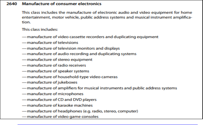
with an ISIC Rev. 4 class (see Box 1, which provides the textual description of the ISIC class
2640 - manufacture of consumer electronics industry).
Box 1. Textual Description of the Manufacture of Consumer
Electronics Industry
Source: International Standard Industrial Classification System of All Economic Activities Rev. 4.

23
The method chosen was the natural language processing (NLP) library word2vec that scores
the Google Trends category / topic description against the ISIC industry class description (at
the 4-digit level). Any Google Trends category that matched to an ISIC industry within a
given threshold is retained (See technical annex for details). The Google Trends by category
are then aggregated using a simple average to the ISIC class. This aggregation is illustrated in
Tables 12 and 13 below.
Table 12. Monthly Google Trends SVIs at ISIC 4-digit level for Accommodation
and Food Service Activities (I) for Australia
At ISIC 4-digit level we take the average Google Trends SVIs of all matched categories.
ISIC 4-
digit
ISIC description
Trends category
description
Trends
category
Jan-
21
Feb-
21
Mar-
21
Apr-
21
May
-21
5610
Accommodation and food
service activities; Food and
beverage service activities;
Restaurants and mobile
food service activities
Food & Drink: 71;
Restaurants: 276;
Fast Food: 918
918 90.0 82.0 85.0 91.0 87.0
5610
Accommodation and food
service activities; Food and
beverage service activities;
Restaurants and mobile
food service activities
Business &
Industrial: 12;
Hospitality
Industry: 955; Food
Service: 957;
Grocery & Food
Retailers: 121
121 70.0 66.0 61.0 73.0 68.0
5610
Accommodation and food
service activities; Food and
beverage service activities;
Restaurants and mobile
food service activities
Business &
Industrial: 12;
Hospitality
Industry: 955; Food
Service: 957;
Restaurant Supply:
816
816* - - - - -
5610
Accommodation and
food service activities;
Food and beverage
service activities;
Restaurants and mobile
food service activities
Total 5610
Average
SVIs
80.0 74.0 73.0 82.0 77.5
5629
Accommodation and food
service activities; Food and
beverage service activities;
Event catering and other
food service activities;
Other food service
activities
Food & Drink: 71;
Restaurants: 276;
Fast Food: 918
918 90.0 82.0 85.0 91.0 87.0
5629
Accommodation and food
service activities; Food and
beverage service activities;
Event catering and other
food service activities;
Other food service
activities
Food & Drink: 71 71 83.0 78.0 74.0 86.0 84.0
5629
Accommodation and
food service activities;
Food and beverage
service activities; Event
catering and other food
Total 5629
Average
SVIs
86.5 80.0 79.5 88.5 85.5

24
ISIC 4-
digit
ISIC description
Trends category
description
Trends
category
Jan-
21
Feb-
21
Mar-
21
Apr-
21
May
-21
service activities; Other
food service activities
5630
Accommodation and food
service activities; Food and
beverage service activities;
Beverage servin g activities
Food & Drink: 71;
Non-Alcoholic
Beverages: 560;
Coffee & Tea: 916
916 92.0 83.0 82.0 93.0 97.0
5630
Accommodation and food
service activities; Food and
beverage service activities;
Beverage servin g activities
Food & Drink: 71;
Non-Alcoholic
Beverages: 560
560 96.0 89.0 83.0 91.0 94.0
5630
Accommodation and food
service activities; Food and
beverage service activities;
Beverage servin g activities
Food & Drink: 71 71 83.0 78.0 74.0 86.0 84.0
5630
Accommodation and
food service activities;
Food and beverage
service activities;
Beverage serving
activities
Total 5630
Average
SVIs
90.3 83.3 79.7 90.0 91.7
* This category did not return data for Australia for this instance. Included for completeness.
Source: Author’s estimates.
Table 13. Monthly Google Trends SVIs at ISIC Section Level for
Accommodation and Food Service Activities (I) for Australia
At ISIC section level we take the average Google Trends SVIs of all matched categories to ISIC 4-
digit removing duplicate categories to keep a simple average.
ISIC 4-
digit
ISIC description
Trend’s category
description
Trend’s
category
Jan-
21
Feb-
21
Mar-
21
Apr-
21
May-
21
5610
Accommodation and food
service activities; Food and
beverage service activities;
Restaurants and mobile
food service activities
Food & Drink: 71;
Restaurants: 276;
Fast Food: 918
918 90.0 82.0 85.0 91.0 87.0
5610
Accommodation and food
service activities; Food and
beverage service activities;
Restaurants and mobile
food service activities
Business &
Industrial: 12;
Hospitality
Industry: 955;
Food Service:
957; Grocery &
Food Retailers:
121
121 70.0 66.0 61.0 73.0 68.0
5610
Accommodation and food
service activities; Food and
beverage service activities;
Restaurants and mobile
food service activities
Business &
Industrial: 12;
Hospitality
Industry: 955;
Food Service:
957; Restaurant
Supply: 816
816 - - - - -
5629
Accommodation and food
service activities; Food and
beverage service activities;
Even t catering and other
food service activities; Other
food service activities
Food & Drink: 71 71 83.0 78.0 74.0 86.0 84.0
5630
Accommodation and food
service activities; Food and
Food & Drink: 71;
Non-Alcoholic
916 92.0 83.0 82.0 93.0 97.0
25
beverage service activities;
Beverage serving activities
Beverages: 560;
Coffee & Tea: 916
5630
Accommodation and food
service activities; Food and
beverage service activities;
Beverage serving activities
Food & Drink: 71;
Non-Alcoholic
Beverages: 560
560 96.0 89.0 83.0 91.0 94.0
Total
Accommodation and food
service activities
Total
Average
SVIs
86.2 79.6 77 86.8 86
Source: Author’s estimates.
The benefit of the Google Trends data is that users have access to a long and high frequency
time series. These data are particularly useful in helping understand turning points and are
intended to be combined with and benchmarked to official measures to improve their
timeliness and frequency. Therefore, the emphasis of the series will generally be on the
current period. While the emphasis is on the current period a long time series is required to
establish relationships and models with existing official measures of economic activity. Since
there are many factors that can influence search intensity a 5-year moving intervals is used
and the weekly trends are smoothed using a five-week moving average. To derive the
monthly and quarterly series the weekly series was averaged for the month or quarter.
Finally, often the series exhibit lag effects and therefore for certain series – such as travel
type series where vacation interest precedes the trip some consideration should be given to
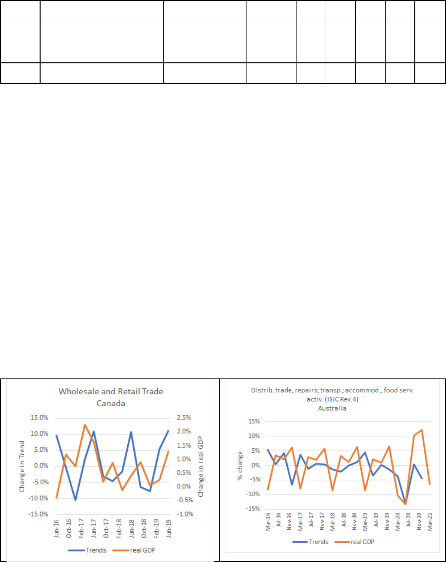
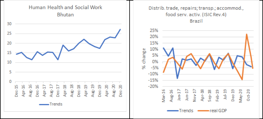
lagging the series. This needs to be done on a case-by-case basis. Figure 6 compares the
Google Trends by ISIC index with real GDP for selected industries for a sample of countries.
In many cases the trends exhibit similar patterns and are very good at predicting the turning
points.
Figure 6. Change in Google Trends Compared to Change in Real Quarterly
GDP (in percentages)
26
Figure 6. Change in Google Trends Compared to Change in Real Quarterly
GDP (in percentages) (continued)
*Note – Bhutan does not release quarterly estimates of GDP.
IV. U
SING GOOGLE DATA FOR GDP NOWCASTING
In this application, we show the predictive ability of our indicators in nowcasting quarterly
GDP for selected industries for a group of countries during the pandemic. Our objective is to
determine if our business activity indicator, operating status indicator, reopening indicator,
and Google Trends by ISIC correlate well with official GDP numbers and can be used to
improve the timeliness and frequency of GDP preliminary estimates through simple
regression techniques. Specifically, we want to show that the strength of these indicators is to
closely track the fall and subsequent rebound of economic activities that were particularly hit
by the effects of the pandemic in the second and third quarter of 2020.
First, we selected a sample of six countries with availability of quarterly GDP data by
economic activity. The selected countries are Australia, Brazil, Canada, France, the
Philippines, and South Africa. The sample is sufficiently heterogenous with respect to
income level, economic structure, and geographic locations. We consider all economic
activities at the one-digit level of the ISIC available from the official statistics agency (e.g.,
19 sections in the ISIC rev. 4). Although longer times series were available for some of these
countries, for this exercise we only considered data from 2015-Q4 to 2020-Q3 to match the
five-year span available for our Trends series by ISIC. All data were used in seasonally
adjusted form. It should be noted that we picked a sample of countries where quarterly GDP
already existed, so that we could test the accuracy of nowcasting at the quarterly level using
the indicators developed in this research. Nevertheless, our indicators can also be used to
produce quarterly estimates of the GDP in those countries where only annual GDP is
available, for example by using annual-to-quarterly benchmarking techniques.
27
We performed a correlation analysis at the 1-digit ISIC level between our Google Trends
series and quarterly Gross Value Added (GVA) by economic activity in the last five years.
Positive (contemporaneous) correlations were found for many ISIC sections in the service
industry for most countries, most notably Transportation and Storage (H), Accommodation
and Food Services activities (I), Professional, Scientific, and Technical activities (M), Arts,
Entertainment and Recreation (R). With few exceptions, correlation for industrial activities
and the primary sector was substantially lower.
Correlation for the “Transportation and Storage” activity was strikingly consistent across
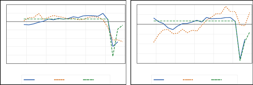
countries, which prompted us to focus our nowcasting exercise on this sector. Figure 7 shows
the official GDP data for section H and the respective Google Trends series for the six
countries in our sample. We also include in the charts the reopening indicator for the last
three quarters of 2020. We found that real Transportation and Storage gross value added
showed high and consistent correlation with the respective Google Trends series for all
countries. Google search categories matched to Transportation were, among others,
“Aviation,” “Freight and Trucking,” “Rail Transport,” “Maritime Transport” and “Public
Storage” We believe that the number of hits of search terms in these categories (e.g., “get an
air ticket to New York”) can track closely the movements of activities related to travel that
were severely hit during the pandemic, such as air, maritime, and railroad transportation and
supporting activities.
Figure 7. Transportation and Storage: Comparison between Official Data
(GDP-H), Google Trends (TRE-H), and Reopening Indicator (REOP) for
Selected Countries
Period: 2015-Q4-2020-Q4. Seasonal adjusted and normalized data.
Australia
Brazil
-5
-4
-3
-2
-1
0
1
2
2015 2016 2017 2018 2019 2020
GDP-H
TRE-H
REOP
-4
-3
-2
-1
0
1
2
2015 2016 2017 2018 2019 2020
GDP-H
TRE-H
REOP
28
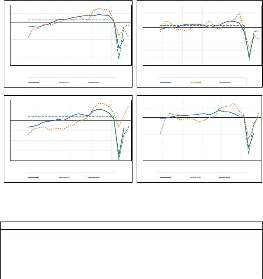
Figure 7. Transportation and Storage: Comparison between Official Data
(GDP-H), Google Trends (TRE-H), and Reopening Indicator (REOP) for
Selected Countries (continued)
Canada
France
The Philippines
South Africa
Table 14. Transportation and Storage: Regression Results
Period: 2015-Q4-2020-Q3.
Regression model in logs, no lags, plus constant. Seasonally adjusted data.
Likewise, our regression results show that both indicators are good predictors of
Transportation and Storage activity. Table 14 shows that the model fitting is very good f o r all
countries, with an R
2
above 80 percent. All models are estimated in logs with a constant
value. Coefficients for both indicators are positive and statistically significant. It is important
to note that the reopening indicator (REOP) is a dummy variable available only for three
quarters (2020-Q2, 2020-Q3, and 2020-Q4.) As shown in Figure 1, the fall and subsequent
-5
-4
-3
-2
-1
0
1
2
2015 2016 2017 2018 2019 2020
G
DP-H
TRE-H
REOP
-5
-4
-3
-2
-1
0
1
2
3
2015 2016 2017 2018 2019 2020
G
DP-H
TRE-H
REOP
-4
-3
-2
-1
0
1
2
2015 2016 2017 2018 2019 2020
GD
P-H
TRE-H
REOP
-5
-4
-3
-2
-1
0
1
2
2015 2016 2017 2018 2019 2020
GDP-H
TRE-H
REOP
Model for GDP-H
TRE-H
REOP
R
2
Coeff.
t-stat
Coeff.
t-stat
Australia
0.83
0.43
3.22**
0.19
2.43**
Brazil
0.91
0.10
2.21**
0.30
13.20**
Canada
0.88
0.89
5.57**
0.38
6.44**
France
0.92
0.25
2.15**
0.48
7.28**
Philippines
0.95
0.45
6.40**
1.28
15.96**
South Africa
0.92
0.25
2.47**
0.34
8.90**
29
rebound of the reopening indicators almost perfectly match the effects of the pandemic noted
in the official data.
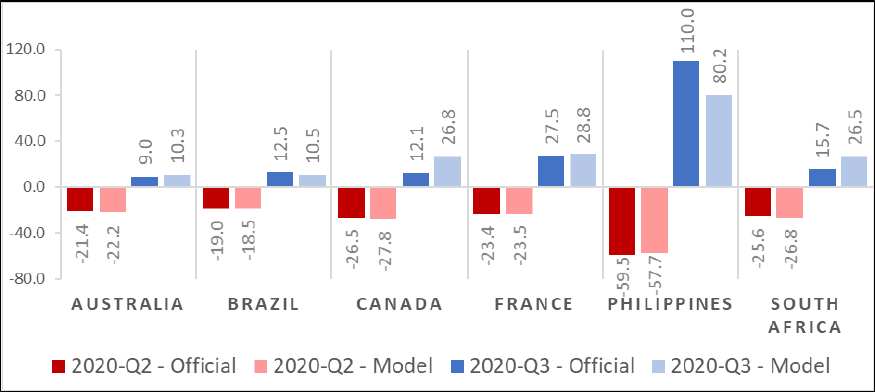
Finally, we used the regression models to produce nowcasts of the second and third quarter
of 2020. Figure 8 compares the official estimates produced by the national statistics agencies
with our model estimates. The large drop in 2020-Q2 is accurately captured by our
predictions, and those for 2020-Q3 adequately anticipate the subsequent recovery. The
advantage of our nowcasts is that they could have been produced a few days after the end of
each quarter, given that the Google data from Trends and Places API are available in real-
time.
Figure 8. Transportation and Storage: Nowcasts for 2020-Q2 and 2020-Q3
Data expressed in quarter-to-quarter rate of change, seasonally adjusted
V. C
ONCLUSIONS
The pandemic highlighted the need to use nontraditional data to prepare more timely and
detailed economic indicators. With the onset of the pandemic, consumption and production
patterns changed dramatically. Consumers rapidly changed their preferences and behaviors,
shifting from traditional brick-and-mortar stores to online shopping. As governments swiftly
passed lockdown measures amid an unprecedented health crisis worldwide, businesses were
forced to close or moved to remote working, when possible. As these dramatic events
unfolded, real-time data on people’s mobility and business-related activities made available
by the private sector played a key public policy function for decision makers and the citizens.
In this work, we developed high-frequency indicators based on Google data to measure the
various business dynamics and activity since the start of the pandemic. First, we used Google
Places API to build indicators of “business status” for several major cities for the period
April 2020 to the current period. Second, we transformed Google Trends data into “business
activity” indicators that match the classifications used in the national accounts and other

30
official business statistics. Through a simple regression experiment, we showed that the two
indicators could predict very well the fall and subsequent recovery in the GDP of selected
countries during the early stage of COVID-19.
Beyond assessing the impact of COVID-19, our purpose was to expand the methodological
toolkit for national statistics agencies and central banks interested in increasing timeliness
and frequency of economic indicators using Google data. The key advantage of Google data
is that they are easily accessible in all countries. Google Trends series can be accessed at no
cost from a publicly available website
maintained by Google. Places API can be used to
retrieve data on the operational status of businesses (and other information) for a small fee,
relative to the cost of collecting the same data through surveys or interviews (when possible).
Countries with significant lags in the production of quarterly national accounts may test these
indicators to release early estimates of quarterly GDP. Countries producing only annual GDP
data may find these indicators useful to produce sub-annual estimates on an experimental
basis for selected sectors of the economy. Quality of these indicators should be tested and
validated with official high-frequency indicators, such as industrial production indexes,
retails sales, and value-added-tax indicators.
We encourage countries to develop experimental high frequency indicators of economic
activity based on our methodology. The technical annex and the R package provided with
this paper can be used to reproduce the step-by-step procedure for building the same
indicators for any country. These indicators will need to be assessed to determine their ability
to nowcast national accounts data and other official indicators available with a long delay. If
these indicators show accurate and robust results vis-à-vis traditional data, countries should
consider publishing experimental products to provide faster signals on the status of the
economy to their users. Investing resources to develop innovative statistical products based
on nontraditional sources will make these countries better equipped and prepared to tackle
the next period of economic turbulence.

31
Annex I. Technical Aspects of Google Trends and Google Places API
This Annex outlines the data collection and processing methods IMF staff (the authors) used
to transform and process the data acquired from the Google Trends Platform and Google
Maps Platform (using the Google Places API).
Google Maps Platform (Google Places API)
Google Places API, part of the Google Maps Platform
, provides developers access to a set of
APIs and SDKs that allows them to embed Google Maps into mobile apps and web pages, or
to retrieve data from Google Maps. The Places API is a service that returns information about
“Places” using HTTP requests. Places are defined within this API as establishments,
geographic locations, or prominent points of interest.
Data collection
For this study, IMF Staff selected a sample of 24 cities (initially, only 13: Bogota, Istanbul,
Lagos, London, Madrid, Manila, Mumbai, New York, Paris, Sao Paulo, Sydney, Tokyo,
Toronto) that were the most affected by the COVID-19 lockdowns
10
representing the world’s
major geographical areas. The authors drew an initial sample of n (<= 60) establishments for
each Places Type
11
by distance from the center of the city.
12
For most “Places Types” the
number of sample units was less than 60 (n < 60 - there will be fewer than 60 “amusement
parks” in any given city). Some businesses have multiple types assigned to them by Google,
(e.g.: a Place can be classified as both “restaurant” and “food delivery”) so the final sample
size n for certain types could be > 60 but was limited to 60 for operational reasons.
For each city, for each type, IMF staff queried the Google Places API 3 times (60 max
responses concatenating 20 max responses per individual query) using search term = type
and latitudes and longitudes of the city center as illustrated below:
sstring = gsub("_"," ",t),
lat = y,
lon = x,
type = t,
num_iter = round(cat_sample_size/20)
The frequency of the data collection has varied since the launch of the project. At the
beginning of the pandemic the aim was to track the evolution of the status of businesses, so
10
https://en.wikipedia.org/wiki/National_responses_to_the_2019%E2%80%9320_coronavirus_pandemic#Lockdowns.
11
full list of 96 types: https://developers.google.com/places/web-service/supported_types?hl=en_US.
12
city centers: https://simplemaps.com/data/world-cities.

32
IMF staff took weekly / bi-weekly samples. Since the COVID-19 lockdowns have subsided
in most countries data are now being collected once per month on the last day of the month.
The following variables are collected with each collection cycle:
Basic Fields
Address Component
Address
Business Status
Formatted Address
Viewport
Location
Icon
Name
Photo
Place ID
Plus Code
Typ e
URL
UTC Of f set
Vicinity
Contact Fields
Phone Number
International Phone Number
Opening Hours
Website
Atmosphere Fields
Price Level
Rating
Reviews
User Ratings Total
A key variable collected is the business status indicator. Google does not provide an
explanation of how they maintain this information but, according to Partoo,
13
they collect
data from many different sources to avoid relying exclusively upon businesses action to
update their businesses status.
Connecting to the Google Places API
Users of the Google Places API require a Google account, typically a Gmail account, and
need to register with Google Cloud: https://cloud.google.com/gcp/getting-started
. Once
registered, users can create a project and select the Google APIs they are interested in using.
For this study the
Places API was selected.
By signing up on Google Cloud and setting up a billing account, each user receives $300 in
credits, which correspond to approximately 170K queries. Depending on the scope of the
13
https://www.partoo.co/en/blog/how-does-the-temporarily-closed-label-work-on-google-my-business/.

33
project this may be sufficient. For our purposes each collection cost $300 (60 establishments
by 96 types by 24 cities at $.0017 per query is $235).
14
This work was generously funded by
Google through the Google Maps Platform credits for crisis responders
.
Data processing and exploration
IMF staff used the googleway
15
package in R
16
to acquire data from the Google Places API.
Once the data was acquired the following variables were extracted from the HTTP request:
business status, place_id, name, icon, city, period, type, geometry.location.lat,
geometry.location.lng, rating, user_ratings_total, price level. IMF Staff then removed
remove potential duplicates of (place_id, type) pairs and merged the data with the city
coordinates file (see previous section, world_cities dataset) and check for outlying latitudes
and longditudes, i.e., avoid places not belonging to the vicinity of the city. This was
accomplished by filtering businesses such that:
lat < lat_city_center + 1 & lat > lat_city_center - 1
and
lng < lng_city_center + 1 & lng > lng_city_center – 1
where we approximate 1 degree of lat/lng to 110 km
17
Lastly, IMF staff imputed for missing periods and assigned an ISIC class.
IMF staff have prepared R code that can be used to replicate the extraction of the data, the
pre-processing and the generation of the indicators. This is provided in Annex II (see the
documentation of the imfgoogle R package).
Google Trends
According to Google Trends FAQs
, Google Trends provides access to a largely unfiltered
sample of actual search requests made to Google. The data are anonymized (no one is
personally identified), categorized (determining the topic for a search query) and aggregated
14
Google recently (as of April 2021) updated their terms and conditions. They are now charging $.032 per
ca ll.
14
15
https://cran.r-project.org/web/packages/googleway/index.html.
16
https://www.r-project.org/.
17
Note: The reason some queries return results outside of the specified location and radius is because when
Google does not f ind a t lea st 20 establishments from a particular location, it will f ill up the resulting da ta with
places in the vicinity of your IP address. If, for instance, you query places API for zoos in Bogota from
Washington DC, you might see the Smithsonian is part of the queried data.

34
(grouped together). This allows Google to display interest in a particular topic from around
the globe or down to city-level geography.
Data Collection
IMF queried data at the country level using the R package gtrendsR
18
that wraps Google
Places API calls. IMF staff queried weekly data for the past 5 years (there was a
methodology change around 2016
19
) at the category level as defined by Google. To obtain
“Trends” for all categories, we are limited by the number of queries for the same IP:
approximately one country every 24 hours. Knowing this limitation imposed by Google,
there are ways to maximize the number of countries returned each day by querying only
those categories and countries of interest. We recommend users try different combinations of
parameters for an optimal data collection strategy.
By default, each query to Google Trends returns 3 different datasets: Trends, Related Topics
and Related Queries. The main measure is called the Search Volume Index (SVI) (for related
topics and queries, this is represented in column “subject”). According to
Google Trends
FAQs: Google Trends normalizes search data to make comparisons between terms easier.
Search results are normalized to the time and location of a query by the following process:
- Each data point is divided by the total searches of the geography and time range it
represents to compare relative popularity. Otherwise, places with the most search
volume would always be ranked highest.
- The resulting numbers are then scaled on a range of 0 to 100 based on a topic’s
proportion to all searches on all topics. See methodology section for a detailed
explanation
Keywords,
20
or related queries, are difficult to use in multi-country analysis, and may suffer
from ambiguities. For example, a search for “Ibiza” could be categorized either in relation to
the Island or the car (Seat Ibiza). With keywords, it is possible to capture changes in
popularity at a very granular level by country and regions, but this approach is time
consuming and requires heavier work on taxonomy and language.
18
https://cran.r-project.org/web/packages/gtrendsR/index.html.
19
For details see: https://www.oecd-ilibra ry.org/economics/tracking-activity-in-real-time-with-google-
trends_6b9c7518-en.
20
The following 3 paragraphs are based on: https://www.oecd-ilibra ry.org/economics/tracking-activity-in-real-
time-with-google-trends_6b9c7518-en.
35
Individual search terms are attributed to categories encompassing words focused on a
common issue. Categories
21
are structured according to a hierarchical classification
developed by Google. Components of a given category are adjusted to prevent double
counting. Categories are comparable across countries and grouping of searches are
constructed using an algorithm that is not disclosed. Using Google Trends categories rather
than keywords allows for a more comprehensive treatment of searches and makes it easier to
compare results across countries. Searches are categorized across detailed groups harmonized
across languages, giving a more comprehensive picture than from a single search term and
allocating terms to an appropriate use. There is also a translation of terms so that searches in
multiple languages are recognized.
Related topics are a collection of keywords terms which include all search terms related to a
specific term. They are also constructed using an algorithm and remove some of the
ambiguity associated with keywords. For some dimensions, opting for a more granular
approach based on topics rather than category can prove more satisfactory to design
meaningful economic indicators.
Sample results: (for a fictitious country XX)
Interest by category
date
Search Volume
Index (SVI)
Geo
Time
group
category
2016-01-31
00:00:00 UTC
97
XX
today+5-y
web
3
2016-02-07
00:00:00 UTC
98
XX
today+5-y
web
3
2016-02-14
00:00:00 UTC
95
XX
today+5-y
web
3
2016-02-21
00:00:00 UTC
94
XX
today+5-y
web
3
2016-02-28
00:00:00 UTC
94
XX
today+5-y
web
3
Related topics
Subject
related_topics
value
Geo
category
100
Top
YouTube
XX
3
32
Top
Film
XX
3
19
Top
MP3
XX
3
11
Top
Gambling
XX
3
11
Top
Download
XX
3
Related queries
Subject
related_queries
Value
geo
category
100
Top
youtube
XX
3
21
https://github.com/pat310/google-trends-api/wiki/Google-Trends-Categories.

36
99
Top
youtube
XX
3
24
top
mp3
XX
3
12
top
mp3 youtube
XX
3
12
top
kristal bet
XX
3
Linking Google Trends categories and ISIC Rev. 4 products
To derive measures of economic activity from Google Trends, IMF staff developed an
algorithm to map the Google-based taxonomies with the ISIC Rev. 4. IMF staff leveraged the
hierarchical structure of Google Trends categories and ISIC Rev 4 four-digit products to
create sentences we could then use as inputs for machine-based text models. The basic steps
are outlined below:
1. Build the hierarchies. For example:
ISIC hierarchy: descriptor (code)
Agriculture, forestry and fishing (A)
Crop and animal production, hunting and related service activities (01)
Growing of non-perennial crops (011)
Growing of sugar cane (0114)
Google Trends hierarchy: descriptor (code)
Business & Industrial (12)
Agriculture & Forestry (46)
Food Production (621)
2. To build the input sentences, IMF staff concatenated the elements in the hierarchy.
Example:
ISIC sentence:
agriculture forestry fishing crop animal production hunting growing non
perennial crops growing sugar cane
Google Trends sentence:
business industrial agriculture forestry food production
3. Transform text into vectors by using a pre-trained embeddings space based on
GloVe,
22
an unsupervised learning algorithm for obtaining vector representations for words.
22
https://nlp.stanford.edu/projects/glove/.

37
Each word is assigned a 50-d vector and, each sentence like the above, is assigned the
average of the 50-d of its words’ vectors
23
4. Once IMF staff transformed sentences into vectors of the same 50-d space, IMF staff
calculated the Euclidean distance or cosine similarity between any of these vectors, and, thus,
compare the similarity of their corresponding texts. Example:
Distance (“agriculture forestry fishing crop animal production hunting
growing non perennial crops growing sugar cane”, “business industrial
agriculture forestry food production”) = 0.863
Note: the higher the Distance measure the closer the match, so this is a similarity
measure, for instance:
Distance (“business industrial agriculture forestry food production”,
“business industrial agriculture forestry food production”) = 1
5. IMF staff were able to follow this approach at any level in the hierarchy. To
compensate for the differences in length and hierarchical depth of the concatenated
sentences, IMF staff computed 3 different vector embeddings, and therefore 3 distances for
each pair of sentences:
a) Complete hierarchy, see above example
b) Top node in the hierarchy. In our example:
Distance (“agriculture forestry fishing”, “business industrial”) = 0.922
c) Bottom element in each hierarchy. In our example:
Distance (“growing sugar cane”, “food production”) = 0.736
6. Finally, for each ISIC sentence we keep the closest 5 Google Trends categories and
compute 2 custom weighted scores to further filter the best matches:
• Weighted sum of distances (0 <= sum_dist_w =< 6). Keep sum_dist_w
>= 4
• Weighted count of the number of distances > .85 (0 <= count_dist_w =<
6). Keep count_dist_w >= 3
Weights were assigned to give extra importance to higher nodes in the hierarchy:
a) Complete hierarchy, weight = 3
b) Top node, weight = 2
23
Note: In our case, we used the 50-dimensional vector space lea rned from the Wikipedia 2014 + Giga word 5
(6B tokens, 400K vocab, uncased).

38
c) Bottom note, weight = 1
Thus, in our example:
sum_dist_w = 3*0.863 + 2*0.922 + 1*0.736 = 4.984
count_dist_w = 3*1 + 2*1 + 1*0 = 4
7. Because the matching is done at the 4-digit ISIC Rev. 4, it allowed IMF Staff to link
ISIC sections (A, B, C, etc.) to a combination of Google Trends categories. This is explained
in the paper and illustrated in tables 10, 11 and 12.
From weekly to monthly Trends by ISIC industries
Once we have a system in place to map Google categories to standard economic
classifications by industry, we can construct practical indicators. As explained in the paper, if
we want to find correlations with standard GDP variables, we may want to transform our
weekly data into monthly or quarterly. Below we explain how to achieve this for the monthly
data:
- Monthly SVIs are calculated as the average of the weekly SVIs for a given category
and country
- Monthly SVIs for ISIC level 4 is the average of the monthly SVIs for matched
categories
- Monthly SVIs for ISIC section is the average of the monthly SVIs for all unique
categories mapped to this section.
For instance, we can plot each of the monthly SVIs by ISIC Rev. 4 at 4-digit and at section
levels:
Figure 1: Monthly SVIs (hits) at ISIC Rev 4 4-digit and section levels for section Q: Human
health and social work activities, from October 2015 to October 2020

39
Similarly, we can compute the growth over time:
Figure 2: Monthly growth SVIs (hits_growth) at ISIC Rev 4 4-digit and section levels for
section Q: Human health and social work activities, from October 2015 to October 2020
Bias and noise reduction
By using this bottom-up approach we achieve a more robust measure of each sector in the
economy. Individual searches may be biased towards a negative or positive sentiment. SVIs
measure how popular a specific search is and, to remove the sentiment bias, it would need to
be complemented by using several SVIs from related words. Fortunately, this is already
taken care of by Google’s Trends categories, which is the focus of our study. Still, if we only
target one category to measure a specific aspect of the economy, we may be getting a biased
sample. This is where our approach could be useful to reduce the noise associated with the

40
SVIs of an individual category by using a combination of several categories to produce an
estimate at the ISIC section level.
Even with the above methodology, there still may be significant sampling noise for smaller
countries for certain categories. Taking multiple samples on a weekly basis and taking the
average of SVIs as the current SVI may reduce this variance as suggested in Woloszko
(2020)
24
Chaining and rescaling
Moving beyond a one-time Google Trends data collection to a production system where we
update SVIs regularly poses some questions which are discussed in this section. For example,
some of the questions we need to consider if we start with an initial 5-year weekly SVIs and
intend to update the data on a weekly basis include:
• Do we query new 5-year data every week for the same countries & categories (T-2
weeks of overlap), or do we aim at querying, say, 1-month worth of data (4 weeks, 3
weeks of overlap) at a daily frequency, which we aggregate to weekly?
• What is the best way to chain 2 SVIs time series? There are different ways we can
rescale the SVIs resulting from the new data, calculating the difference, the ratio, the
ratio between ranges, etc. Does this matter? Do we need to rescale the whole series or
just add the new data point at the end based on one of the rescaling options?
According to Woloszko (2020), the rescaling needs to be multiplicative. The definition of an
SVI is: #searches (“car”)/#searches (all) * const., where the constant is here to ensure that the
max = 100. So, two SVIs covering different time ranges may have different const, as the max
of the relative search intensities can occur at two different points in time:
SVI_a = #searches (“car”)/#searches (all) * const_a
in theory:
SVI_a * SVI_b/SVI_a = #searches (“car”)/#searches (all) * const_b.
But this is only true in theory, because each SVI is computed over a fixed-rate sample of the
universe of Google Searches. That is the second cause of existing differences between SVI_a
and SVI_b. As a result, rescaling SVI_a over SVI_b using the ratio between the two series
based on only one observation is probably not a good idea. A possible solution would be to
multiply SVI_b by the mean of the ratio of SVI_a/SVI_b taken over all common
observations.
24
"Tra cking a ctivity in rea l tim e with Google Trends," OECD Economics Department Working Papers, No.
1634, OECD Publishing, Paris, https://doi.org/10.1787/6b9c7518-en
.

41
Annex II. Data and Methods with the imfgoogle R Package
This annex explains how to install and use the ‘imfgoogle’ package in R, which the authors
created to implement the techniques used in this working paper.
A. Install and load imfgoogle
Place the binary source package in the R library folder of your local computer, typically:
C:/R/R-3.6.3/library/. You need to have R installed in your local computer and the location
of your R library folder may be different, depending on the R version or the operative
system. Next start R or RStudio and run:
> install.packages("C:/R/R-3.6.3/library/imfgoogle_0.1.0.tar.gz",
repos = NULL, type="source")
> library(imfgoogle)
B. Available datasets
imfgoogle includes several datasets used throughout the paper. To access any of them simply
run:
> data(“name_of_dataset”)
The following datasets are included in the R package:
• Trends_categories_codes_full_hierarchy
Google Trends categories with indentation and full hierarchy
category indentation categCode full_categCode
All categories: 0 1 0 ;0
Arts & Entertainment: 3 2 3 ;3
Celebrities & Entertainment News: 184 3 184 ;3;184
Comics & Animation: 316 3 316 ;3;316
…
• ISIC_4d_full_hierarchy
ISIC Rev. 4 complete hierarchy
isicCode Description indentation
full_isicCode
A Agriculture, forestry and fishing 2 A
01 Crop and animal production, hunting and related service activities 3 A;01
011 Growing of non-perennial crops 4 A;01;011
0111 Growing of cereals (except rice), leguminous crops and oil seeds 5
A;01;011;0111
…
• Google_Places_types_ISIC_NAICS
Google Places types matched with ISIC and NAICS products

42
type isic_codes isic_code_label isic_secti
on
bakery 1061 1062 Manufacture of starches and starch products C
roofing_contractor 4100 410 4100 Construction of buildings F
plumber 4322 4322 Plumbing, heat and air-conditioning installation F
car_dealer 4530 453 4530 Sale of motor vehicle parts and accessories G
…
• mapping_isic4d_trendsCategories
ISIC Rev. 4 products matched to Google Trends categories as used in the paper to
compute Google Trends SVIs at ISIC section level
isicCode categoryCode dist_full dist_top dist_bottom
0111 749 0.8849943 0.9223012 0.8423424
0112 621 0.8711644 0.9223012 0.7637744
0113 749 0.8592794 0.9223012 0.7195353
0114 621 0.8631717 0.9223012 0.7358893
…
• match_Trends_categories_ISIC_products
Distances (cosine similarity) between Google Trends categories and ISIC Rev. 4
products greater or equal than 0.8
category isic_product dis
t
arts entertainment arts entertainment recreation 0.9
53
arts entertainment arts entertainment recreation creative arts entertainment 0.9
85
arts entertainment arts entertainment recreation libraries archives museums cultural 0.8
73
…
• cities_places
List of select cities used to collect Google Places API
C. Methods
Operating Status Indicators
The Google Places API permits users to extract the operating status of each place identified
on the Google Places platform. Places are given the status of “Open”, “Temporarily Closed”
or “Permanently Closed”. This information can be used to produce several useful business
dynamic indicators.
Operational Indicator
The operational index represents the share of Places in a given geographic region that are
operational at a given point in time weighted by the number of reviews. The R function
below generates the indicator as described in the paper:

43
biz_status_places(
in_data_path = ".",
out_data_path = ".",
file_prefix = "sample_Google_places_",
city_pop_limit = 1e+06,
sample_freq = "month",
write_out = TRUE
)
The following example saves an Excel file to the specified out_data_path parameter location:
biz_status_places(in_data_path = "C:/Users/<MyUserName>/Box Sync/Google
Places API/data/", out_data_path = "<output_directory>")
Here is an excerpt:
status city placetype period statuso statuswo
<chr>
<chr>
<chr>
<chr>
<dbl>
<dbl>
1 OPERATIONAL Atlanta Total 2020-05-30 93.4 90.6
2 OPERATIONAL Atlanta Total 2020-07-26 96.1 96.5
3 OPERATIONAL Atlanta Total 2020-08-26 98.3 98.1
4 OPERATIONAL Atlanta Total 2020-09-17 98.5 97.5
5 OPERATIONAL Atlanta Total 2020-10-17 98.8 98.6
6 OPERATIONAL Atlanta Total 2020-11-25 98.6 98.4
…
Business Re-opening Indicator
This indicator is used to track the path and pace at which businesses that are temporarily
closed in a region re-open. The R function below generates the indicator as described in the
paper:
biz_reopening_places(
in_data_path = ".",
out_data_path = ".",
exclude_periods = c("2020-06-29"),
select_cities = NULL,
longitudinal = FALSE,
groupby_var = "city",
method = "reopening",
interpolate = FALSE,
min_sample_size = 50,
write_out = TRUE
)
The following example returns a data.frame with the reopening indicator for the select group
of cities as illustrated in the table in Figure 4 of the paper:
reopening_isicSection <- biz_reopening_places(in_data_path =
"C:/Users/<MyUserName>/Box Sync/Google Places API/data/")
This indicator can be generated for different aggregations: by Google Places type, ISIC or
NAICS. For example, running the following will generate the reopening indicator aggregated
at ISIC Rev. 4 section: A, B, C, …

44
reopening_isicSection <- biz_reopening_places(in_data_path =
"C:/Users/<MyUserName>/Box Sync/Google Places API/data/",
groupby_var = "ISIC_section")
And this will aggregate by Google Places business type for a specific city:
reopening_isicSection <- biz_reopening_places(in_data_path =
"C:/Users/<MyUserName>/Box Sync/Google Places API/data/",
groupby_var = "type", select_cities = "Manila")
Business Activity Indicators
Google Trends capture the interest in a topic relative to all other topics at a given point in
time. If we assume that there is a relationship between changes in interest in a topic(s) and
changes in business activity the Google Trends could be used as a proxy for business activity
(at least in the short term). Similarly, the Google Places API permits users to extract reviews
from the Google Places platform.
Google Reviews as an indicator of business activity
For this indicator, the rating was used to adjust the number of reviews such that a Place with
100 poorly rated reviews would have a lower weight than a Place with 100 highly rated
reviews. Since the maximum score for a review is 5 the “adjusted” number of reviews was
calculated as (average rate / 5) *(number of reviews).
biz_reviews_places(
in_data_path = ".",
out_data_path = ".",
file_prefix = "sample_Google_places_",
city_pop_limit = 1e+06,
sample_freq = "month",
write_out = TRUE
)
To generate the underlying data for Figure 5 outlined in the paper simply run:
biz_reviews_places(in_data_path = "C:/Users/<MyUserName>/Box
Sync/Google Places API/data/", out_data_path = "<output_directory>")
Here is an excerpt of the output file:
city placetype wr2020-04-24S1 wr2020-05-30S1 wr2020-05-30S2 wr2020-06-
20S2
Baghdad accounting 206.76 209.50 NA NA
Baghdad airport 1946.30 2018.96 NA NA
Baghdad amusement_park 3946.60 3996.86 NA NA
Baghdad aquarium 10714.18 10826.10 NA NA
…
Google Trends as an indicator of activity
45
Calculates Google Trends for ISIC Rev. 4 different industry levels. This method allows users
to generate Tables 12, 13 and Figure 6 as shown in the paper.
biz_activity_trends(
out_data_path = ".",
select_countries = NULL,
select_categories = NULL,
select_isic_sectors = NULL,
select_keyword = NA,
only_interest = FALSE,
time_span = "today+5-y",
write_out = TRUE
)
The following example calculates weekly SVIs and related topics and queries for ISIC Rev.4
sector "A" (Agriculture, forestry and fishing), for the past 5 years from Spain's web searches:
biz_activity_trends(out_data_path = "C:/Users/<MyUserName>/Box
Sync/Google Places API/data/", select_isic_sectors = c("A"),
select_countries = c("ES"))
As described in the paper, this approach “links” the textual information underscoring a
specific Google category / topic with the textual information associated with a specific ISIC
class. Readers may find the file mapping categories and ISIC codes by loading the
mapping_isic4d_trendsCategories dataset included in the imfgoogle package by running:
> data(“mapping_isic4d_trendsCategories”)
This file already selects the best matches according to criteria explained above. However, the
package also includes a dataset with the distances (cosine similarity) between Google Trends
categories and ISIC Rev. 4 products greater or equal than 0.8. To load this dataset:
> data(“match_Trends_categories_ISIC_products”)
Finally, users also have the possibility to run alternative mappings using the imfgoogle
package. The following function returns, in its default choice of parameter values, the
mapping dataset described above and utilized in this paper as reference:
match_categ_trends(
refresh = FALSE,
dist_threshold = 0.8,
custom_dist_threshold = 0.85,
removeDup = FALSE,
keepTop_n = 5,
weight_score = 4,
count_score = 3
)

46
However, by setting the refresh parameter to TRUE and selecting different values for the rest
of the parameters, it is possible to obtain an alternative mapping file. See technical annex
above for a full explanation of this method.
D. References
Some of the methods and datasets included in this annex benefited from the following
valuable sources:
- World cities: https://simplemaps.com/data/world-cities
. Free version under Creative
Commons Attribution 4.0
- Pre-trained word vectors from Wikipedia 2014 + Gigaword5: glove6B under Public
Domain Dedication and License v1.0. For more information on GloVe:
Jeffrey Pennington, Richard Socher, and Christopher D. Manning. 2014. GloVe:
Global Vectors for Word Representation. [pdf] [bib]
- googleway R package. Under MIT + file LICENSE
- gtrendsR R package. Under GPL-2 | GPL-3 [expanded from: GPL (≥ 2)]
47
REFERENCES
Abraham, K., R.S. Jarmin, B. Moyer, and M.D. Shapiro (editors), 2019, Big Data for
Twenty-First Century Economic Statistics: Proceedings of Conference held in March
2019, (National Bureau of Economic Research Series: Studies in Income and Wealth,
University of Chicago Press).
Bank for International Settlements, 2021, “Use of Big Data Sources and Applications at
Central Banks,” Irving Fisher Committee on Central Bank Statistics, February 2021.
Choi, H., and H. Varian (2012), “Predicting the Present with Google Trends”, The Economic
Record, Volume 88 Special Issue, June 2012, pp.2-9.
Elvidge, C.D., K.E. Baugh, E.A. Kihn, H.W. Kroehl, E.R. Davis, and C.W. Davis, 1997,
“Relation between satellite observed visible-near infrared emissions, population,
economic activity and electric power consumption,” International Journal of Remote
Sensing, Volume 18, Issue 6, pp. 1373-1379.
Jun, S., H. Yoo, and S. Choi, 2018, “Ten Years Research Change Using Google Trends:
From the Perspective of Big Data Utilizations and Applications” Technological
Forecasting and Social Change Vol. 130, pp.69-87.
M. Luca, 2016, “Reviews, Reputation, and Revenue: The Case of Yelp.com,” Harvard
Business School Working Paper 12-016.
Narita, F., and R. Yin, 2018, “In Search of Information: Use of Google Trends' Data to
Narrow Information Gaps for Low-income Developing Countries,” IMF Working
Paper 18/286 (Washington: International Monetary Fund).
Schmidt, T., and S. Vosen, 2011, “Forecasting Private Consumption: Survey-based
Indicators vs. Google Trends,” Journal of Forecasting 30, no. 6 (September 2011):
pp.565-578.
OECD Issue Note:1: The OECD Weekly Tracker of activity based on Google Trends.
