
Climate Impacts to Restoration
Practices – Project Report
September 18, 2020
PREPARED FOR
PREPARED BY
Sadie Drescher
Director, Restoration Programs
Chesapeake Bay Trust
108 Severn Avenue,
Annapolis, MD 21403
(410) 974-2941 x105
Jonathan Butcher
Tetra Tech
One Park Drive, Suite 200
PO Box 14409
Research Triangle Park, NC 27709
(919) 485-8278
Contributing authors
Scott Job, Nancy Roth, Bryan Groza, Brian
Pickard, and Peter Kwon
CBT Request #16928, Deliverable # 11
100-IWM-T39881
2
This page left intentionally blank

IDF Project Report September 2020
i
CONTENTS
EXECUTIVE SUMMARY .............................................................................................................................. 1
1.0 INTRODUCTION ..................................................................................................................................... 5
2.0 METHODS .............................................................................................................................................. 7
2.1 Statistical Theory .............................................................................................................................. 8
2.1.1 IDF Updates ............................................................................................................................ 8
2.1.2 Peaks over Threshold Analysis for Sub-yearly Events ......................................................... 11
2.2 Runoff and BMP Simulation with SWMM ....................................................................................... 14
2.2.1 Bioretention ........................................................................................................................... 16
2.2.2 Extended Wet Detention Basin ............................................................................................. 16
2.2.3 BMP Sizing with Maryland Environmental Site Design......................................................... 17
3.0 DATA .................................................................................................................................................... 19
3.1 NOAA IDF Curve Stations in Maryland .......................................................................................... 19
3.2 Climate Model Selection ................................................................................................................. 21
4.0 RESULTS – EXTREME PRECIPITATION ........................................................................................... 37
5.0 RESULTS – EVENT RUNOFF AND BMP SIMULATIONS ................................................................. 41
5.1 Runoff ............................................................................................................................................. 41
5.2 Bioretention BMP ............................................................................................................................ 42
5.3 Extended Wet Detention BMP ........................................................................................................ 47
6.0 IMPLICATIONS FOR DESIGN ............................................................................................................. 51
6.1 Channel Stability ............................................................................................................................. 51
6.2 Roadway Flooding Risk .................................................................................................................. 58
6.3 Urban BMP Performance ............................................................................................................... 67
6.3.1 BMP Systems: Environmental Site Design ........................................................................... 68
6.3.2 Design of Individual Practices ............................................................................................... 72
7.0 DISCUSSION ........................................................................................................................................ 75
7.1 Potential Use of Continuous Simulation ......................................................................................... 75
7.2 Adaptation of BMPs in a Changing Climate ................................................................................... 76
7.3 Stream Restoration Design Considerations ................................................................................... 78
8.0 REFERENCES ...................................................................................................................................... 81
APPENDIX A. PYTHON CODE ............................................................................................................. 89
A-1. IDF Updates ................................................................................................................................. 89

IDF Project Report September 2020
ii
A-2. Peaks-over-Threshold Analysis ................................................................................................. 108
A-3. SWMM Simulations .................................................................................................................... 120
TABLES
Table 2-1. Curve Numbers for Environmental Site Design Simulations (MDE, 2009)............................... 18
Table 3-1. Key to NOAA Atlas 14 Sites ..................................................................................................... 20
Table 3-2. Key to CMIP5 GCM Scenarios in the LOCA Downscaled Climate Data Archive ..................... 23
Table 3-3. Bounding Scenarios for Analysis of Changes in Precipitation Volume, ca. 2056 .................... 24
Table 3-4. Bounding Scenarios for Analysis of Changes in Precipitation Volume, ca. 2085 .................... 27
Table 3-5. Bounding Scenarios for Analysis of the 90
th
Percentile 24-hour Precipitation Event, ca. 2056 30
Table 3-6. Bounding Scenarios for Analysis of the 90
th
Percentile 24-hour Precipitation Event, ca. 2085 33
Table 5-1. Summary of Response of Bioretention to 90
th
-percentile Event ............................................... 43
Table 5-2. Summary of Responses of Bioretention to Future 1-year through 100-year Events ................ 44
Table 5-3. Summary of Response of Extended Wet Detention to 90
th
-percentile Event ........................... 47
Table 5-4. Summary of Responses of Extended Wet Detention to Future 1-year through 100-year Events
....................................................................................................................................................... 48
Table 6-1. Probability of Channel Instability for Runoff from 1 Acre with S/√d
50
= 1.75, with and without
Bioretention BMPs ......................................................................................................................... 55
Table 6-2. Probability of Channel Instability for Runoff from 1 Acre Parcel with Alternative S/√d
50
at 80%
Imperviousness .............................................................................................................................. 55
Table 6-3. Probability of Channel Instability for Runoff from 25-Acre Parcel based on 1-yr 24-hr Event
with Alternative Values of S/√d
50
.................................................................................................... 58
Table 6-4. HY-8 Results, Local Road Culvert ............................................................................................ 63
Table 6-5. HY-8 Results, Minor Arterial Culvert ......................................................................................... 64
Table 6-6. Polynomial Coefficients for Relationship of Headwater Elevation and Outlet Velocity to Flow 66
Table 6-7. Curve Numbers for Environmental Site Design Simulations .................................................... 69
Table 6-8. Treatment Volume (Q
E
, inches) for Historic and Predicted Future Climate for Hydrologic Group
D Soils, Developed Land at 80% Imperviousness ......................................................................... 70
Table 6-9. Relationship of Excess Stormwater Volume to Q
E
Calculated using Environmental Site Design
Procedure from 2009 Design Manual (MDE, 2009) – Hydrologic Soil Group A ............................ 70
Table 6-10. Relationship of Excess Stormwater Volume to Q
E
Calculated using Environmental Site
Design Procedure from 2009 Design Manual (MDE, 2009) – Hydrologic Soil Group B ................ 71
Table 6-11. Relationship of Excess Stormwater Volume to Q
E
Calculated using Environmental Site
Design Procedure from 2009 Design Manual (MDE, 2009) – Hydrologic Soil Group C ............... 71
Table 6-12. Relationship of Excess Stormwater Volume to Q
E
Calculated using Environmental Site
Design Procedure from 2009 Design Manual (MDE, 2009) – Hydrologic Soil Group D ............... 72

IDF Project Report September 2020
iii
FIGURES
Figure 2-1. Threshold Value Detected by the Python Algorithm for Site 18-7140 ..................................... 14
Figure 2-2. Future 90
th
-percentile Rainfall Event Predictions for Different GCMs at Site 18-7140 ........... 14
Figure 2-3. Schematic of IDF Analysis Tool ............................................................................................... 15
Figure 2-4. Curve Number Prediction of Runoff as a Function of Precipitation for Hydrologic Group D
Soils, Developed Land at 80% Imperviousness ............................................................................ 18
Figure 3-1. NOAA Atlas 14 Sites in Maryland and the District of Columbia .............................................. 19
Figure 3-2. Example Biplot of Forecast Changes in Average Annual Precipitation and Air Temperature for
Durham North Carolina for 2050 - 2080 vs. 1950 – 2005 .............................................................. 21
Figure 4-1. Projected 25-year IDF Curves for Baltimore WSO Airport ca. 2055 ....................................... 38
Figure 4-2. Projected 25-year IDF Curves for Baltimore WSO Airport ca. 2085 ....................................... 39
Figure 4-3. Projected Results for 90
th
Percentile 24-hour Precipitation Event, Aberdeen-Phillips Field ... 40
Figure 5-1. Historic and Future Peak Flow Averages by Recurrence ....................................................... 42
Figure 5-2. Bioretention Simulation Results for Peak Outflow as a Function of Total Storm Depth .......... 45
Figure 5-3. Bioretention Simulation Results for Overflow Volume as a Function of Total Storm Depth.... 46
Figure 5-4. Extended Wet Detention Basin Simulation Results for Peak Outflow as a Function of Total
Storm Depth ................................................................................................................................... 49
Figure 5-5. Extended Wet Detention Simulation Results for Overflow Volume as a Function of Total
Storm Depth ................................................................................................................................... 50
Figure 6-1. Stability Transition Frontier for Sand Bed Stream with 1-acre Drainage................................. 53
Figure 6-2. Average Mobility Index for 25% (left) and 80% (right) Impervious Cover 1-acre Parcel, S/√d
50
= 1.75 m
-0.5
..................................................................................................................................... 54
Figure 6-3. Predicted Probability of Channel Instability at 25% Imperviousness for Runoff from a 1 Acre
Site with S/√d
50
= 1.75 using the Logistic Regression of Bledsoe and Watson (2001) ................. 54
Figure 6-4. Histogram of Individual Station/GCM/Imperviousness for Probability of Channel Instability
with S/√d
50
= 1.75, 1 Acre Drainage, and no BMP ......................................................................... 56
Figure 6-5. Inverse Cumulative Distribution Function (Percentage Greater than Specified Level) of
Individual Station/GCM/Imperviousness for Probability of Channel Instability with S/√d
50
= 1.75, 1
Acre Drainage, and no BMP .......................................................................................................... 56
Figure 6-6. Average Mobility Index for 25% (left) and 80% (right) Impervious Cover, 25-acre Parcel,
S/√d
50
= 0.35 m
-0.5
.......................................................................................................................... 57
Figure 6-7. Average Mobility Index for 80% Impervious Cover, 25-acre Parcel, S/√d
50
= 0.35 m
-0.5
(left)
and S/√d
50
= 1.0 m
-0.5
(right) ........................................................................................................... 57
Figure 6-8. Minor Arterial Road Culvert, HY-8 Specifications .................................................................... 60
Figure 6-9. Local Road Culvert HY-8 Specifications ................................................................................. 61
Figure 6-10. Relationship between Peak Flow from 1-acre (80% Impervious) and 24-hour Precipitation
Depth .............................................................................................................................................. 62
Figure 6-11. Relationship of Headwater Elevation and Outlet Velocity to Flow for Local Road (Left) and
Minor Arterial (Right) Culvert Designs ........................................................................................... 65
Figure 6-12. Predicted Frequency of Road Overtopping under Future Climate, Local Road Culvert ....... 66
Figure 6-13. Predicted Frequency of Road Overtopping under Future Climate, Minor Arterial Culvert .... 67
Figure 6-14. Curve Number Prediction of Runoff as a Function of Precipitation for Hydrologic Group D
Soils, Developed Land at 80% Imperviousness ............................................................................ 69
IDF Project Report September 2020
iv
(This page left intentionally blank.)

IDF Project Report September 2020
r 1
EXECUTIVE SUMMARY
Intense precipitation events are increasing in the mid-Atlantic region and climate models suggest this
trend may continue. We derive projections of future extreme precipitation and runoff events throughout
Maryland. These suggest that infrastructure sized to handle historic weather may be inadequate in future
and that urban stream channels may become less stable; however, pollutant removal functions of
stormwater best management practices appear less likely to be adversely affected.
Warmer air can hold more precipitable water and associated potential energy. A warming climate can
thus increase the risk of extreme rainfall events. Recent observations document an increased frequency
of extreme rainfall events throughout the eastern United States and in the Chesapeake Bay watershed.
Climate models generally predict that these trends will continue. However, there is also considerable
uncertainty about the practical implications of these predicted trends for designers and planners. First it
is not precipitation itself, but the runoff generated by precipitation that is of most concern to the
performance of stormwater infrastructure and the protection of stream channel integrity. Further, while a
general trend of increases in extreme precipitation events is well supported by broad spatial averages
over the ensemble of multiple climate model runs, predicted results at specific locations and in individual
climate models can be quite different from one another.
In many U.S. jurisdictions, including Maryland, designs for stormwater infrastructure rely on estimates of
the recurrence interval or frequency (F) of a storm of a given intensity (I) and duration (D) – the so-called
IDF curve. For example, regulations might require that a minor road culvert be designed to pass the flow
resulting from the precipitation associated with the 24-hour storm event that would reoccur, on average,
once every 25 years. The National Oceanic and Atmospheric Administration (NOAA) has published IDF
curves for weather stations throughout most of the U.S. For Maryland, these IDF curves are developed
by a statistical extreme value fit to series of annual maximum daily precipitation recorded through
December 2000.
Use of the NOAA IDF curves implicitly assumes that weather observed through 2000 is applicable to
current and future conditions. The evidence already suggests that changes in the IDF relationships have
occurred since 2000, while climate models predict continuing changes.
How can we account for such changes, especially regarding future conditions that may be encountered
during the design life of a project? Global climate models have limited skill at predicting extreme
precipitation events. For one, many of the most intensive rainfall events are associated with convective
storms that occur at spatial scales that are smaller than the grid size of global climate models and with
tropical storm events that are inherently difficult to predict. One potential solution is to use a regional
weather model to predict more local responses when used with the global climate model providing
boundary conditions. This is an informative exercise, but different regional models also differ, further
increasing the multiplicity and potentially the range of results. More importantly, regional models are
computationally expensive to run. The Coupled Model Intercomparison Project of the World Climate
Research Programme in its most recently completed 5
th
round of experiments (CMIP5) includes output
from over 32 different global climate models, each of which was run for at least two greenhouse gas
forcing scenarios and it is not readily feasible to run all these permutations through a regional model –
especially as the results of the new CMIP6 updated runs are now becoming available.
For this project we take a different, more computationally efficient approach to evaluating IDF curves
consistent with CMIP5 global climate results. Essentially, we ask the question “What would the NOAA

IDF Project Report September 2020
r 2
IDF curves look like if they had been calculated from annual maximum precipitation series that had been
modified to reflect changes in climate conditions indicated by the global climate models?” To do this we
first make use of readily available climate prediction series that have already been downscaled to a
smaller spatial scale and a daily time step. This is done using a “constructed analogs” approach, in which
a library of historical observation series is used to scale from a monthly to a daily time step, ensuring a
reasonable representation of the temporal structure of local rainfall, coupled with a spatial bias correction
step based on comparison to historic observations that reduces the spatial size of the output grid to 1/16
degree (approximately 6.9 x 5.4 km at the latitude of Baltimore).
Our approach does not assume that the downscaled global climate models are able to provide accurate
estimates of future extreme rainfall events. Rather, we assume that, for a given global climate model, the
relative change between historic and future conditions for events of a given recurrence can be used to
assess the likely change in the annual maxima series used to develop NOAA’s IDF curves. We then re-fit
the extreme value distribution to the revised maxima series to generate a climate modified IDF curve.
This method is computationally efficient and allows us to generate potential future IDF relationships using
multiple climate models at all 74 Maryland stations for which NOAA has published IDF curves.
Design of “green” management practices for water quality treatment is often based on retaining the runoff
from the 90
th
or 95
th
percentile (i.e., sub-yearly) 24-hour precipitation event. The IDF analysis based on
annual maxima series is not applicable to sub-yearly events. However, a similar updating procedure was
constructed on a peaks-over-threshold analysis. A database containing estimates of future IDF curves
and 90
th
percentile events was constructed for all 74 Maryland stations analyzed by NOAA. For each
station this includes estimates of conditions centered at 2055 and 2085 from four different climate
models, selected to represent a drier case (10
th
percentile of all models in total rainfall volume), a wetter
case (90
th
percentile), and two cases near the median for a low and a high greenhouse gas emissions
scenario.
Results of the IDF analysis suggest a widespread risk under future conditions of increased intensity of
extreme precipitation events of a given duration and recurrence. However, this increase is not consistent
among GCM scenarios downscaled by LOCA, with some models predicting drier conditions with a lesser
frequency of extreme rainfall events. Consistent changes were not predicted in the magnitude of the 90
th
percentile event. This is in line with studies that suggest total annual precipitation volume will most likely
increase under future climate, but that much of this increase will be associated with more extreme, low-
recurrence events. The 90
th
percentile results thus appear to be “good news” as they suggest that many
water quality best management practices (BMPs) that are optimized to capture and treat pollutants
associated with sub-yearly recurrence events are likely to continue to provide expected services under
future climate.
Once estimates of the precipitation distributions are obtained it is necessary to calculate runoff. This was
done by routing the precipitation through EPA’s Storm Water Management Model (SWMM) using a
generic unit-area representation of an urban landscape with varying levels of impervious. SWMM was
also used to represent performance of bioretention cells and extended wet detention pond BMPs,
representative of green and gray approaches to stormwater management.
As with precipitation, there is a wide range of predictions from different climate models and different
stations for extreme runoff. However, by the end of the century, peak runoff rates are predicted to
increase, on average, about 13 – 14 percent, with slightly higher increases for longer recurrence intervals
and lower impervious percentages.

IDF Project Report September 2020
r 3
Both bioretention and extended wet detention BMPs tended, on average, to produce less outflow and
lower peak flows in response to the 90
th
percentile event under future climate. However, for large, longer
recurrence events future predictions include increased peak flows and a larger volume of flow that
overflowed or bypassed the BMP.
We undertook three additional analyses to evaluate practical consequence of these predicted changes in
precipitation and runoff:
• Channel Stability and Stream Restoration Design: Stream restoration design seeks to create
stable, resilient channels. Stability is highly site-specific and, in addition to runoff, depends on
channel substrate, slope, and existing morphology. However, analysis of stability indices for
channel-forming flows suggest that changes in IDF relationships will increase the risk that some
streams will shift from stable to unstable conditions.
• Roadway Flooding Risk and Culvert Design: Undersized culverts are a common cause of
hazardous road overtopping during high flow events. Maryland specifies design standards for
culverts based on road class and service life. For example, a culvert on a local road must be
designed to safely pass the peak runoff from a 10-year 24-hour storm and has a minimum service
life goal of 50 years. Model simulations suggest that a culvert designed for the current 10-year
storm may have, on average, a risk of overtopping of about 15% by 2055 and a risk of 37% by
2085. This may indicate a need to revise design standards to address nearer-term conditions
and the possible need for a larger culvert at the end of the 50-year service life.
• BMP Performance Efficiency: The Maryland Department of the Environment has adopted an
Environmental Site Design approach for new development under which the combination of BMPs
on a site needs to control runoff in response to the 1-year 24-hour storm so that it is no greater
than the runoff that would be expected for the same site with a cover of undeveloped woods in
good condition. We examined how these design criteria might fare under future climate and
found that only a small increase in risk is anticipated on average, largely because the projected
changes in the 1-year event are small.
Adaptation to a changing climate is challenging because models, while numerous, are uncertain, there is
no single best predictor of the future, and the course of climate response will depend on human political
and economic decisions. Exercises like this report help inform us about the range of risks that may need
to be faced but deciding where to balance risk and cost is inherently political. What is clear is that it is
preferable to employ solutions that are resilient and adaptable – able to perform well under a variety of
future conditions and amenable to be adjusted with low regret costs if the future is not as predicted. In
this context, stormwater management using green components such as bioretention that can be
expanded or altered as needed are likely preferable to gray infrastructure such as retention basins that, if
they turn out to be undersized, are difficult and expensive to replace. Low-regret opportunities that
benefit resource management regardless of whether and how climate changes are preferable.
For climate-smart stream restoration design, resilience and adaptability should be explicit objectives.
Maintaining floodplain connectivity is one key to building natural resilience and designs should anticipate
greater uncertainty in the flow regime, not just increases in large events. The overall goal is to maximize
the ability of the stream to adjust gradually to a range of potential, but uncertain, hydrometeorological
changes over the design life of the project.

IDF Project Report September 2020
r 4
(This page left intentionally blank.)

IDF Project Report September 2020
r 5
1.0 INTRODUCTION
Engineering design for stormwater management is largely based on empirical evidence obtained from
past data with the assumption that the frequency of extreme events that is likely to be seen in the future
can be inferred from the historical record. This implies that climate is stationary; however, in many
regions of the U.S., the intensity and frequency of major precipitation events is projected to increase
(Hayhoe et al., 2018). Predicted changes in future climate imply the end of the assumption of stationarity
that has provided the foundation of water management for decades, as was announced by Milly et al.
(2008). Commenting on the “death of stationarity”, Galloway (2011) noted “there is also a great need to
provide those in the field the information they require now to plan, design, and operate today’s projects.”
Kunkel et al. (2013) identified increasing trends in the number of 2-dau precipitation events exceeding a
once-in-five-year threshold throughout the eastern half of the U.S. Easterling et al. (2017) in the Fourth
National Climate Assessment reported changes in both the number and magnitude of large precipitation
events. Hoerling et al. (2016) looked at precipitation above the 95
th
percentile daily event and found
consistent increases in the Northeast but not in the Southeast U.S. (Maryland is on the border between
the two regions). Howarth et al. (2019) summarize recent observations for the Northeast U.S. and
identified statistically significant increases in the top one percent of daily rainfall events. Expected
increases in the frequency of intense rain events in the Chesapeake Bay watershed is supported by the
4th National Climate Assessment (Dupigny-Giroux et al., 2018). Thibeault and Seth (2014) and Lynch et
al. (2016) also document recent observed and future projected increases in intense rain events in the
area.
Design of urban stormwater BMPs typically begins with consideration of rainfall recurrence intervals,
which may be translated into design storm specifications or runoff depth. Practices are designed to
achieve a level of service or performance associated with controlling a certain design storm, combination
of design storms, and/or runoff depth to reduce flooding, stream erosion, and pollutant loading. In most
areas, design standards for BMPs incorporate sizing requirements based on storms of a specified
intensity, duration, and frequency (IDF analysis). The performance of stormwater practices is dictated
primarily by precipitation IDF, impervious surface area, and soils, along with life cycle maintenance
(Berndtsson, 2010; Claytor and Schueler, 1996; Gallo et al., 2012, Hunt et al., 2012, Kadlec and Knight,
1996, Khan et al., 2012; Roseen et al., 2009). If the IDF relationships change, the design standards for
both gray and green infrastructure components should change as well to preserve retention capacity and
treatment contact times that are essential to treatment efficiency.
IDF curves graphically summarize the relationship between precipitation intensity and the duration of
precipitation events for a given frequency or recurrence interval. IDF curves provide important
information for engineering design and planning purposes. From one perspective, updating IDF curves
for future climate is simple – conditional on reliable estimates of the distribution of future precipitation
events. Unfortunately, the skill of GCMs in predicting individual precipitation events is limited, especially
convective storm events that provide the most intense storms yet occur at spatial scales smaller than the
resolution of GCMs. For light precipitation, GCMs tend to overestimate the frequency but reproduce the
observed patterns of intensity relatively well. For heavy precipitation, GCMs roughly reproduce the
observed frequency, but underestimate the intensity (Sun et al. 2006; Sillmann et al. 2013; Mehran et al.
2014). Some of the biases inherent in GCMs are resolved by downscaling results to a finer, local scale,
often with a bias correction step. However, Maraun et al. (2010) conclude that serious deficiencies

IDF Project Report September 2020
r 6
remain in the ability of downscaling methods to generate local precipitation series with the correct
temporal variability.
For most of the U.S. (including Maryland), estimates of precipitation frequency at pre-defined recurrence
intervals of once per year through once per 1,000 years for specific weather observation stations are
provided as IDF curves and tables in the National Oceanic and Atmospheric Administration (NOAA)’s
Atlas 14 (e.g., Perica et al., 2013) and companion Precipitation Frequency Data Server
(https://hdsc.nws.noaa.gov/hdsc/pfds/). A specific objective of the work described in this report is to
provide a method to update Atlas 14 IDF curves to reflect potential future changes in model-predicted
local climate. To satisfy this objective it is important to understand the way in which the Atlas 14
estimates were created.
Frequency estimates in Atlas 14 are based on fitting an extreme value distribution (in most cases, a
generalized extreme value [GEV] distribution) to the time series of annual maximum precipitation (AMP)
amounts at a station for seventeen durations ranging from 15 minutes to 60 days. The AMP series
consists of one measurement per year (the largest depth observed for a given duration) and does not
account for the possibility of more than one event in a year exceeding a threshold of interest. The true
probability of occurrence of events of a given intensity and duration should be derived from the partial
duration series, which includes all events of a specified duration and above a pre-defined volume
threshold. Frequency estimates for partial duration series were developed by NOAA for Atlas 14 from the
series of AMPs using Langbein’s conversion formula, which transforms a partial duration series-based
average recurrence interval (ARI) to an annual exceedance probability (AEP):
Equation 1
Selected partial duration ARIs are first converted to AEPs using this formula, and frequency estimates
were then calculated for the AEP using the GEV fit to annual maxima.
For Atlas 14, NOAA fit the GEV for each station using the method of L-moments (Hosking and Wallis,
1997), incorporating regionalization across approximately the 10 nearest stations for higher order L-
moments. NOAA does not release the fitted coefficients of the GEV distribution, although the AMP series
are provided via ftp server. Because the NOAA method is ultimately based only on annual maxima (the
AMP series), only AMPs are needed for future climate conditions and not the complete time series. The
theoretical basis for updating Atlas 14 IDF curves is presented in Section 2.1.
Storms of more frequent occurrence than once per year are also relevant to BMP and restoration design
but cannot be reliably analyzed from AMPs alone. Analysis of these more frequent storms requires a
somewhat different “peaks over threshold” approach, as is also described in Section 2.10.
The size of precipitation events is generally of less direct concern than the amount of runoff produced by
the event, which in addition to precipitation, depends on antecedent moisture conditions, the extent to
which the landscape produces direct runoff (which is closely related to the amount of impervious surfaces
that are present), and the degree to which management practices retain or infiltrate stormwater.
Evaluating runoff requires combining precipitation estimates with a rainfall-runoff model (Section 2.2).
These tools are combined with climate model projections (Section 3.0) to produce precipitation and runoff
results under future climate for Atlas 14 stations throughout Maryland (Sections 4.0 and 5.0). The
remaining sections investigate how projected changes may affect aspects of stormwater infrastructure
design and stream restoration activities

IDF Project Report September 2020
r 7
2.0 METHODS
Updating the IDF curves in Atlas 14 or similar statistical estimates of large precipitation events for future
climate requires understanding how the extreme value distribution fit to annual maximum precipitation
series may change. Over the past two decades – and especially since the 2008 call-to-arms of Milly et al.
– numerous researchers have explored methods for predicting future changes in extreme precipitation
and IDF relationships. While many different methods have been used, all have in common a recognition
that the current generation of GCMs has relatively low skill in predicting extreme precipitation events,
especially those associated with convective storms, which occur at scales smaller than GCM grids. In
essence, predicting extreme precipitation events is a specific form of the general problem of downscaling
from global models that produce monthly-scale climate projections to place-based predictions at daily and
sub-daily time scales. Research in this field falls into four general classes (with terminology in part
adapted from Arnbjerg-Nielsen et al., 2013):
1. Conditional Probability (weather generators): One response to the deficiencies in GCM
simulation of extreme events is to not use the GCM output directly at all, but rather to use
information from the GCMs to populate statistical weather generators, which are then used to
estimate meteorological time-series at the desired spatial and temporal resolution. Conditional
probability methods for precipitation have long been in use for spatial analyses and were adopted
for evaluation of climate response by Fowler et al., (2005), Kilsby et al. (2007), Prodanovic and
SImonovic (2007), and Onof and Arnbjerg-Nielsen (2009). The method remains popular for areas
that lack long term rainfall data (e.g., Shrestha et al., 2017). A fundamental challenge of this
approach is determining the short duration statistical moments of the weather generator from
GCM output that does not provide the necessary temporal resolution
2. Empirical Transfer Functions: Another approach that avoids direct use of GCM precipitation
output is to develop a surrogate relationship between extreme precipitation and other GCM
outputs that are presumed to be predicted with greater accuracy. For example, Willems and Vrac
(2011) developed transfer functions based on atmospheric pressure, while Dahm et al. (2019)
developed an approach to project rainfall extremes by scaling the empirical relationship to
dewpoint temperature. While promising, this approach appears to require development of
transfer function relationships on a site by site basis to obtain robust predictions.
3. Dynamical Downscaling (Regional Climate Models): An alternative approach to improving
rainfall projections for future climate is to use GCM output as boundary conditions to drive a
smaller-scale regional climate model (RCM), or even smaller scale local area model (LAM) that
presumably has better predictive capabilities for local rainfall events. This approach is known as
dynamical downscaling. Future precipitation time series are typically obtained directly from the
RCM or LAM output. Use of dynamical downscaling for precipitation extreme analysis has
soared in popularity with the increasing availability of RCM output produced as part of the
CORDEX (Coordinated Regional Climate Downscaling Experiment; http://www.cordex.org/) effort.
Examples include Rosenberg et al. (2010), DeGaetano and Castellano (2017), Li et al. (2017),
Lettenmaier et al. (2017), Vu et al. (2018), Kristvik et al. (2019), and Cannon and Innocenti
(2019). The advantages of this approach depend on the level of accuracy that is achieved by the
smaller-scale model. One problem with direct use of RCMs is that they generally still do not
explicitly model small-scale cloud processes that cause intense convective storms, for which
LAMs with horizontal scales finer than about 3 km may be needed (Arnbjerg-Nielsen et al., 2013).

IDF Project Report September 2020
r 8
Validation of these models is required before they can be used as input for local climate change
impact studies (Arnbjerg-Nielsen et al., 2013). Further, dynamical downscaling is a time-
consuming process, and results at the RCM scale are not available for many GCMs, much less
LAM analyses.
4. Statistical Downscaling: In recent years, statistical approaches to downscaling have become
widely available. Statistical downscaling is based on relationships that interpolate large-scale
GCM output to observations of historical weather and climate (Wood et al., 2004; Maurer et al.,
2007). Recent advances in statistical downscaling, such as the LOCA (Pierce et al., 2014) and
MACA (Abatzoglou and Brown, 2012) archives, use a constructed analogs approach, in which a
library of historical observation series is used to scale from monthly to daily time step, ensuring a
reasonable representation of the temporal structure of local rainfall. The downscaling process
incorporates a bias correction step and ensures that local, daily time series projections exhibit
patterns similar to historical observed data. This achieves a spatial resolution of 1/6 degree
(approximately 6.9 x 5.4 km at the latitude of Baltimore). The LOCA downscaling approach was
developed to address some shortcomings of the older bias-correction constructed analog
approaches to avoid damping of local precipitation extremes. Statistically downscaled time series
from a GCM could be used to directly estimate IDF relationships or used to describe the relative
change in the extreme value distribution underlying the IDF relationship (e.g., Srivastav et al.,
2014a), as described below. A potential refinement of the approach is to select the downscaling
analogs specifically on the basis of representation of extreme precipitation events (Castellano
and DeGaetano, 2017; DeGaetano and Castellano, 2017; So et al., 2017). The refined approach
focusing on extreme values appears promising but has not been implemented on a national
basis. Any statistical downscaling approach is subject to the caveat of an implicit assumption that
it assumes historical spatial relationships between GCM output and local climate will remain
unchanged over time (Nover et al., 2016).
Some authors have also suggested that the whole framework of IDF curves, with assumption of constant
or stationary parameters (conditional on climate) is misguided and that it is instead preferable to use an
extreme value distribution with non-stationary parameters that could be derived either empirically (based
on observations) or in reference to climate models. This type of approach is combined with Bayesian
conditioning and uncertainty analysis by Cheng and AghaKouchak (2014), and Ragno et al. (2018); see
also Huard et al. (2010).
2.1 STATISTICAL THEORY
2.1.1 IDF Updates
Many of the approaches described above for downscaling precipitation extremes are complex and require
detailed site-specific analyses. Which approach is theoretically optimal for prediction appears to remain
an open question. Our intention here is to use methods that are efficient, use widely available statistically
downscaled data, are consistent with Atlas 14 procedures and results that are incorporated into many
local regulations and design guides, and are model agnostic. A simple, computationally efficient
approach to updating IDF curves was proposed by Srivastav et al. (2014a, 2014b). Their insight was that
the essence of the problem was the need to update extreme value distributions for future conditions, and
that this could be done through a direct analysis of the distributions. The general concept of the approach
of Srivastav et al. (2014a) is described as follows: “…quantile-mapping functions can be directly applied

IDF Project Report September 2020
r 9
to establish the statistical relationship between the AMPs of a GCM and sub-daily observed data rather
than using complete records. Further, the IDF is a distributional function; therefore, it would be easy to
derive the functional relationships between the distributions of the GCM AMPs and sub-daily observed
data. One way of deriving such relationship is by using quantile-mapping functions.”
Quantile mapping (QM) methods, otherwise known as cumulative distribution function (CDF) matching
methods, have long been used as a method to correct for local biases in GCM output. The method first
establishes a statistical relationship or transfer function between model outputs and historical
observations, then applies the transfer function to future model projections (Panofsky and Brier, 1968)
and has been successfully used as a downscaling method in various climate impact studies (e.g., Hayhoe
et al., 2004).
Using the notation of Li et al. (2010), for a climate variable x, the QM method for finding the bias-adjusted
future value of a climate variable can be written as:
Equation 2
where F is the CDF of either the observations (o) or model (m) for observed current climate (c) or future
projected climate (p), and F
-1
is the inverse of the cumulative distribution function. The bias correction for
a future period is thus done by finding the corresponding percentile values for these future projection
points in the CDF of the model for current observations, then locating the observed values for the same
CDF values of the observations.
A significant weakness of the QM method is that it assumes that the climate CDF does not change much
over time, and that, as the mean changes, the variance and skew do not change, which is likely not true
(e.g., Milly et al., 2008). To address these issues, Li et al. (2010) proposed the equidistant quantile
mapping (EQM) method, which incorporates additional information from the CDF of the model projection.
The method assumes that the difference between the model and observed value during the current
calibration period also applies to the future period; however, the difference between the shape of the
CDFs for the future and historic periods is also taken into account. This is written as:
Equation 3
where the form and parameters of the CDF are not yet specified. Srivastav et al. (2014a) argue for using
EQM to update IDF curves; however, the specific method of Srivastav et al. (2014b) is not directly
applicable to updating Atlas 14 IDF curves in the US for several reasons:
• Bias-corrected statistically downscaled climate model output were not widely available for
Canada; therefore, the Srivastav et al. (2014a) method must also incorporate a spatial
downscaling step from the coarse scale of GCMs, whereas output that is already spatially
downscaled to a fine resolution grid is readily available for the US.
• The method of Srivastav et al. justifies use of EQM, but largely consists of a multi-step QM
procedure, without full implementation of the EQM corrections proposed by Li et al. (2010).
• Canada assumes that the AMP series follows a Gumbel, rather than the GEV distribution that is
mostly commonly used in the U.S.
To address these issues, we re-derived under contract with USEPA an EQM method that is consistent
with U.S. design guidelines and makes use of statistically downscaled climate data readily available from
GCM output.

IDF Project Report September 2020
r 10
Our approach uses a combination of EQM and QM to update IDF curves for any location conditional on
output of GCMs for future climate conditions, implemented in Python code. The EQM approach can be
used to update IDF curves for any location conditional on downscaled output of GCMs for future climate
conditions. The process begins with GCM output that has already been subject to spatial bias correction
and downscaling to a finer spatial scale. The calculation step consists of additional spatial downscaling
from the climate output grid to the specific point location of a weather station used by Atlas 14 along with
bias correction for the AMP series (as distinct from the general bias correction of the complete
precipitation series) using the EQM method for different time durations from sub-hourly to daily.
The historical data for this analysis are the historical AMP series used by Atlas 14 (
). Model data
include the predicted AMP series from 1950 to 2005 as historical period (
) and future period (e.g.,
2050- 2080, centered at 2065) of interest (
). A GEV distribution is fit to each of these series,
using the L-moments method (Hosking and Wallis, 1997; implemented in Python in lmoments3 v1.0.4
[Hollebrandse et al., 2015]), consistent with Atlas 14 methods.
To apply the EQM method, quantiles of modeled future AMP series are matched to the distribution for
historical AMPs. For a given percentile, it is assumed that the difference between the model and
observed value also applies to the future period. There are two EQM factors as in Equation 3. The first
is:
,
Equation 4
where the vertical bar “|” indicates conditional dependence, i.e.,
indicates the
cumulative distribution function (GEV for this case) of the future GCM AMP series calculated at the
cumulative probability corresponding to
using the parameter set
calculated for that future
series.
represents the GEV parameters from fit to the Atlas 14 AMP series. To account for the
difference between the CDFs for the model outputs of future and current periods, a second adjustment
factor is calculated:
Equation 5
The projected AMP series is then calculated as:
Equation 6
Once this series is calculated, a GEV fit is applied to estimate the full distribution of the future extreme
events for the local station. This EQM step is applied to update the 24-hour IDF curves. We include
corrections for constrained data (i.e., results for a given duration that are artificially truncated by crossing
over the midnight boundary) using the Atlas 14 factors at this step. The CDFs and inverse CDFs of the
GEV and other extreme value distributions are provided by the lmoments3 Python library.
The second step in adjusting the IDF curves is temporal downscaling to convert future daily extremes into
sub-daily extremes. The QM method was used for this purpose: First find the corresponding percentile
values for these future projection points in the CDF of the model for the historical period, then locate the
observed values for the same CDF values of the sub-daily observations. For rainfall duration i:
Equation 7
As noted in later volumes of Atlas 14 (e.g., Perica et al., 2013), estimates for shorter durations can be
noisy due to limited data availability and are improved by smoothing. To account for the short modeling

IDF Project Report September 2020
r 11
simulation period, the modeled extreme values with less than 24 hours’ duration are thus smoothed by
fitting them to a linear regression relative to the daily maximum series before fitting them to the GEV
distribution. Atlas 14 uses a regression with an intercept for this purpose:
Equation 8
Equation 9
We found that for some Maryland stations the recommended smoothing step could produce negative
estimates of AMS depths. This was resolved by switching to a zero-intercept regression in which b
1
and
b
2
are constrained to be zero.
The adjusted model predictions (
) are then used to fit the GEV distribution with the L-moments
method, and the model predicted partial duration series (PDS) series were retrieved from the derived
GEV distribution at given annual exceedance probability (AEP).
Equation 10
In cases where there are discrepancies between different sub-daily durations (e.g., the 1-hour estimate is
greater than the 2-hour estimate), Atlas 14 suggests maintaining consistency by increasing the estimate
for the longer return interval. This proved problematic because the shorter sub-daily durations (often
estimated from limited data at a station) are much less stable than the daily estimates (which typically
have long runs of data), especially for high recurrence intervals. We revised the approach by enforcing
consistency from the more stable daily estimates downwards to the shorter intervals. For example, if the
1-hour estimate was greater than the 2-hour estimate we reduced the 1-hour estimate rather than
increasing the 2-hour estimate.
The final future 1 to 24-hour IDF ordinates are estimated by multiplying the Atlas 14 published values by
the ratio of fitted GEV PDS results for climate-adjusted future conditions to the fitted GEV PDS results
obtained for the Atlas 14 observed data:
Equation 11
This last step adjusts for the regional representation of higher L moments that is incorporated in the
original Atlas 14 calculations but not explicitly documented for individual stations.
2.1.2 Peaks over Threshold Analysis for Sub-yearly Events
The IDF procedures described above are applicable to storm events with a return period of 1 year or
greater and is most relevant to flood and channel stability analyses. For water quality, design of
individual management practices for water quality treatment is most commonly based on more frequent
events, such as the 90
th
percentile 24-hour rainfall event. The distribution of a sub-yearly event can be
analyzed in a manner analogous to the AMP series for IDF. The primary difference is that the distribution
of the 90
th
percentile event can be described by a Peaks-over-Threshold (POT) approach, which
characterizes the frequency of events greater than a specified magnitude (Serinaldi and Kilsby, 2014).
As the value of the threshold (u) increases, the distribution of the POT (prob Y = (X-u)|X > u) converges to
a generalized Pareto distribution (GPD; Pickands, 1975; Balkema and de Haan, 1974):
Equation 12

IDF Project Report September 2020
r 12
in which {y: y > 0 and
and
, μ is the location parameter, σ > 0 is the scale
parameter, and ξ is the shape parameter. An EQM updating procedure for the GPD, analogous to that
described above for the GEV distribution using H(y) and its inverse, was developed to estimate the
distribution of future 90
th
percentile events and map the changes implied in historic and future GCM runs
onto historic data.
Unlike the AMP analysis, the POT analysis requires working with a complete series of daily precipitation
depths, along with multiple iterations to determine the appropriate threshold for the analysis of events.
Precipitation gauge series typically have missing or accumulated data, which complicate the automation
of the analysis. As with the IDF analysis, we address this issue by using PRISM daily gridded
precipitation estimates that are fit to observed records but filled to provide complete “observed” time
series with bias correction (http://prism.oregonstate.edu).
An important issue for the POT analysis is determining the appropriated threshold for the GPD, which can
have a significant influence on the analysis of precipitation records. A review by Langousis et al. (2016)
found that methods of determining the threshold based on GPD asymptotic properties can lead to
unrealistically high threshold and shape parameter estimates, while nonparametric methods found in the
literature were generally unreliable. Much better results were obtained using the graphical Mean
Residual Life Plot method (Davison and Smith, 1990). In this method, the proper threshold for the GPD
analysis is obtained by plotting the mean of the excesses as a function of the threshold and identifying the
lowest threshold above which the number of excesses increases linearly with the threshold value. While
this method has generally been interpreted graphically, Langousis et al. (2016) provide a method for
automating threshold detection from a continuous daily precipitation time series:
1. Estimate the mean value of the excesses e(u) = E[X-u|X>u] above different thresholds u
i
= Xi,n,
i=1, 2, . . ., n-10, where X
i,n
denotes the ith (ascending) order statistic in a sample of size n.
2. For each u
i
(i=1, 2, . . ., n - 20) in Step 1, apply weighted least squares to fit a linear model to all
points (uj, e(uj)) that satisfy j ≥ i. To account for the increase of the estimation variance of e(u)
with increasing threshold u, the weight w
j
applied to each point (u
j
, e(u
j
)) is taken to be inversely
proportional to the variance of e(u), assuming independence of the excesses. In this case, w
j
=
(n-j)/Var[X-u
j
|X > u
j
].
3. Determine the optimal threshold u* as the lowest threshold u
i
(i=1, 2, . . ., n-20) that corresponds
to a local minimum of the weighted mean square error function of the linear regression,
Once the threshold (u) of historical daily rainfall extracted from PRISM dataset is detected by the
automatic method. The same threshold is applied to daily rainfall series of historical and future predicted
by GCMs. Truncated historical and modeled data(X>u) will be used to predict the changes of 90
th
percentile rainfall magnitude with the EQM methods. To apply the EQM method, quantiles of modeled
future daily rainfall series are matched to the distribution for historical daily rainfall series.
,
Equation 13
where the vertical bar “|” indicates conditional dependence, i.e.,
indicates the
cumulative distribution function (GPD with threshold u for this case) of the future GCM truncated daily
rainfall series calculated at the cumulative probability corresponding to
using the parameter set
calculated for that future series.
represents the GPD parameters from fit to the PRISM
daily rainfall series. To account for the difference between the CDFs for the model outputs of future and
current periods, a second adjustment factor is calculated:

IDF Project Report September 2020
r 13
Equation 14
The projected AMP series is then calculated as:
Equation 15
Then the derived future daily rainfall series
can be fit to GPD distribution. Equation 16 was
used to estimate an unconditional distribution and return value:
Equation 16
where
could be estimated using the ratio between length of rainfall records above threshold
and the full rainfall records. After the probabilities and amounts of rainfall from unconditional distribution
were derived using Equation5. The 90
th
percentile rainfall amount estimated by each GCM was
calculated using linear interpolation:
Equation 17
where Y
90+
and Y
90-
are the observations closest above and below the 90
th
percentile in the rainfall series.
The POT analysis addresses 24-hr events only, so sub-daily analysis is not needed. We do the analysis
using daily rainfall depths without constraint correction [adjustment for events that pass through the day
boundary] as this is the method commonly used in practice to estimate water quality volumes.
We tested the method through preliminary applications to NOAA Atlas 14 station in Maryland. A major
challenge was that the automated selection of the threshold followed by GPD fitting did not always work
properly and sometimes yielded unreasonable results, especially when a very high threshold was
selected. We found that this problem could be solved by providing initial guesses for the parameters of
the GPD distribution that are in the reasonable range for what is obtained for stations with more stable
distributions.
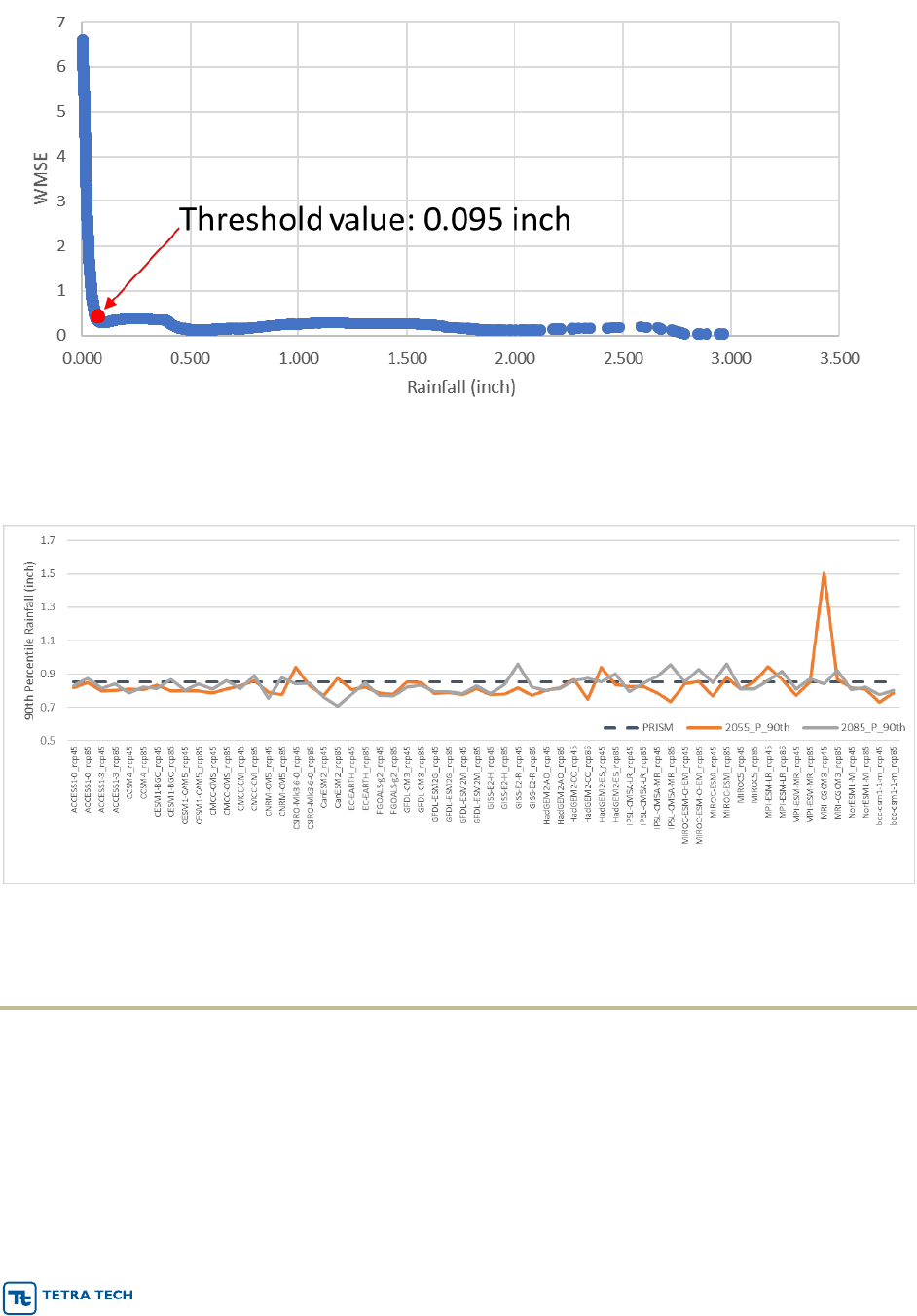
An example of applying the code is shown for Pocomoke City (station 18-7140). The threshold detection
method (Figure 2-1) shows the algorithm successfully estimated the rainfall magnitude at the first local
minimum of weighted mean square error (WMSE). Figure 2-2 is an example of 90
th
percentile rainfall
predictions using all archived GCMs (both rcp45 and rcp85) for 2055 and 2085.
One interesting result of screening analyses across the full set of Maryland Atlas 14 stations is that the
90
th
percentile event may not be predicted to increase, even while a majority of scenarios predict an
increase in total precipitation volume.
While total annual precipitation volume is expected to increase across the Eastern U.S. under future
climate, it is also anticipated that an increasing proportion of annual precipitation will be concentrated in
larger, more intense events (Kundzewicz et al., 2007; Groisman et al., 2012). Future climate may
incorporate both more extreme flood events and longer drought periods, resulting in a situation in which
the 2- to 500-year storm event magnitudes increase, but the 90
th
percentile events decrease. This may
be good news in the sense that BMPs designed to treat water quality in typical storm events (e.g., about
10 times per year) may be adequately sized to address future climate, even though flood control
responses to extreme large events may be inadequate.
IDF Project Report September 2020
r 14
Figure 2-1. Threshold Value Detected by the Python Algorithm for Site 18-7140
Figure 2-2. Future 90
th
-percentile Rainfall Event Predictions for Different GCMs at Site 18-7140
2.2 RUNOFF AND BMP SIMULATION WITH SWMM
Precipitation estimates are converted to runoff with EPA’s Storm Water Management Model version 5
(SWMM5; Rossman, 2015). To evaluate potential runoff depth on a unit-area basis we route the future
storms implied by the IDF curves through the SWMM model (version 5.1.013), packaged in a Python
wrapper with GUI that controls input and output. The actual SWMM subbasin layout needed to
accomplish this task is quite simple. We specify a single BMP catchment (<10 acres and thus not
requiring time of concentration adjustments) for which the user can specify impervious and pervious
acreage, roughness, depression storage, and soil/slope properties. The resulting runoff timeseries can
IDF Project Report September 2020
r 15
be analyzed directly or routed through a variety of gray and green stormwater BMPs, which are explicitly
set up using SWMM input templates.
The IDF curve results are converted into design storm precipitation events for use by SWMM by applying
the appropriate 24-hr rainfall distribution type identified for the Soil Conservation Service TR-55 method
(SCS, 1986). Other, more sophisticated methods of rainfall disaggregation could be used, but we chose
this older method because it is the approach of choice for many local stormwater design manuals.
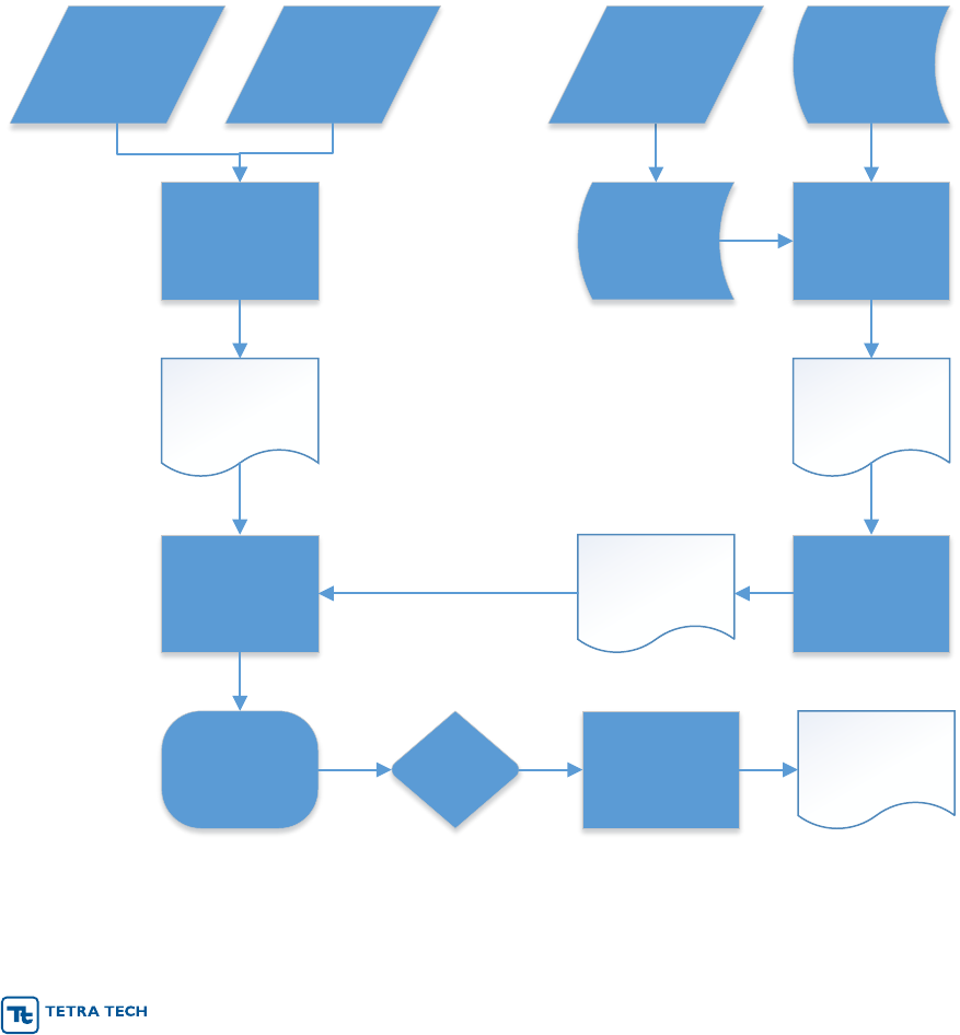
The linkage between the IDF simulations and SWMM is summarized schematically in Figure 2-3. The
IDF analysis portion of the tool appears on the right side. After identification of bounding climate
scenarios (described in Section3.2), the program queries various data servers and retrieves historic and
future climate model output for a user-identified location of interest, along with the AMP series for the
NOAA Atlas 14 station closest to the user location.
All the components of the system are implemented in Python 3. The simulation code is provided in the
Appendix.
User
Input
SWMM
Template
Python
Wrapper
SWMM Input
File
SWMM5
Engine
Climate
Scenarios
IDF Tool
Future IDF and
POT Analysis
Disaggregate
Tool
Design Storms
SWMM
Output
Python
Postprocessor
Results
GCM
Selection
Atlas 14
Existing IDF
Baseline and
BMP
Simulations
Figure 2-3. Schematic of IDF Analysis Tool
For the project we built BMP templates to address a stormwater extended wet detention basin
(representative of a “gray” engineered storage-based management component), and a planted

IDF Project Report September 2020
r 16
bioretention cell (representative of a “green” stormwater infrastructure component that relies on infiltration
and evapotranspiration of stormwater). The next two subsections outline the specifications for
representation of these BMPs:
2.2.1 Bioretention
The generic specification for bioretention includes a 9-inch surface ponding depth, 24 inches of growing
media, and 12 inches of stone drainage layer. The system is assumed to have an underdrain (4-inch
pipe in the middle of drainage layer that controls outflow. The growing media consists of 25% compost
and 75% sandy soil with a porosity of 0.529 (Fassman-Beck et al., 2015). The drainage layer has a void
ratio of 0.54 and a drainage coefficient of 0.18 fir a drain height of 41 inches and drain time of 72 hours.
Storage volume includes the ponding depth and the storage in the media (taking porosity into account).
The depth of storage is thus 0.75 ft ponding + 2 ft media x 0.529 porosity = 1.808 ft.
Maryland uses pre-calculated estimates of WQv and specifies two “rainfall zones” – a western zone and
eastern zone that use a 0.9 in storm and 1.0 in storm respectively for the WQv calculation. As a result,
the assumed bioretention footprint for a given percent impervious area varies by rainfall zone. This was
incorporated by assigning each of the 79 Atlas 14 weather station locations to its corresponding rainfall
zone, and the bioretention footprints were adjusted accordingly.
In addition, we follow Maryland guidance relative to the following:
• Footprint relative to the design treatment volume
• Ponding depth, media depth, and underdrain stone storage layer depth
• Media composition, which influences porosity, infiltration rate, and hydrologic performance
• Underdrain offset from the bottom of the stone storage layer
• Drain time from a completely full state
2.2.2 Extended Wet Detention Basin
The Maryland design for wet ponds assumes that untreated runoff will flow into the pond and displace
“clean” water from the previous storm which has been stored long enough to allow settling and some
nutrient uptake to take place. The untreated runoff enters the pond at one end, and the treated water
exits the other end with minimal mixing of the two (an assumption often referred to as “plug flow”). While
the validity of the plug flow assumption is open to debate, the concept is incorporated into numerous pond
design specifications throughout the U. S. Maryland requires that the permanent pool volume is at least
as large as the treatment volume. In addition to having a WQv requirement, Maryland also specifies a
recharge volume requirement (REv), a relatively smaller fraction of the WQv that must be infiltrated
onsite. Since wet ponds cannot be used to address the REv, we assume the REv has been addressed
on the site upstream of the wet pond. As a result, the wet pond pool volume is assumed to be the
difference between the WQv and the REv. We then increased the pool volume by 10%, in part to be
conservative and also because we did not include any recharge BMPs in the simulation upstream of the
wet ponds.
Our wet pond representation incorporates design guidance for side slopes, including within the pool,
safety and aquatic benches, and the storage basin. An average slope of 34% (run/rise 2.9) was used to
simplify volume calculations. We used pyramid sections to develop the stage-area curves used by
SWMM for the dynamic stage-volume-discharge simulation.

IDF Project Report September 2020
r 17
Maryland also specifies a Channel Protection Volume (CPv), which is specified as extended detention of
the 1-yr 24-hr storm event. Maryland defines extended detention as 12 hours or 24 hours depending on
the Water Use classification of the receiving water. The stormwater manual provides a specific method
for calculating the CPv, the allowable peak discharge for the CPv, and the orifice diameter for the
allowable peak discharge. We incorporated all elements of the specifications for each of the 79 Atlas 14
locations, including WQv Rainfall Zone, Water Use classification, and 1-yr 24-hr storm depth (provided in
the manual by county). The wet pond design also incorporates an emergency spillway to safety pass the
peak flow from the 100-yr 24-hr storm event without overtopping the storage basin.
2.2.3 BMP Sizing with Maryland Environmental Site Design
Implicit assumptions about climate are built into guidance and regulations for both systems of BMPs and
the design of individual BMP types. Maryland Department of the Environment’s (MDE) 2000 Stormwater
Design Manual presented calculations for a Water Quality volume (WQv) and a channel protection
volume (CPv) for the design of stormwater BMPs. With the 2009 revisions to the Design Manual, MDE
moved to the more holistic approach of Environmental Site Design (ESD), which combines the WQv and
CPv objectives to produce a unified approach to stormwater design and management based on the net
effects of all stormwater controls present on a site (MDE, 2009, Chapter 5).
The general concept of ESD is to control runoff from a developed site in response to the 1-year 24-hour
storm so that it is no greater than the runoff that would be expected for the same site with a cover of
undeveloped woods in good condition, considering the distribution of hydrologic soil groups on the site.
ESD does not require detailed simulation modeling of developed and undeveloped conditions. Rather, it
provides a simplified approach based on the relative change in Curve Number used in the National
Resources Conservation Service TR-55 method (NRCS, 1986). The difference in responses to the 1-yr
24-hr event determines the excess runoff that needs to be treated (Q
E
). In units of depth, Q
E
= P
E
x R
V
.
R
V
is the surface runoff fraction, defined as R
V
= 0.005 + 0.009 x I, where I is the impervious fraction
expressed as a percentage. P
E
is then the excess rainfall amount that needs to be treated. Rather than
calculating P
E
, simple lookup tables are provided (one for each of the four hydrologic soil groups, A, B, C,
and D). P
E
is listed in the table in increments of 0.2 inches and imperviousness in increments of 5% and
incorporates a single assumption about the 1-yr 24-hr storm across all of Maryland, so the answer is not
exact, but is sufficient to achieve the desired level of control on average, especially when weighted across
multiple subareas of a site with differing soil and development characteristics.
The approach of controlling site runoff to levels expected for woods in good condition is in theory climate
agnostic because both developed and woods runoff will change if climate changes. However, the table
that is used to determine P
E
is rooted in specific assumptions about the magnitude of the 1-yr 24-hr storm
event that may not hold under future climate conditions.
We investigated this issue by examining the changes in precipitation and the resulting difference in runoff
between developed and good condition woods, as predicted by TR-55, under future climate scenarios for
the 79 NOAA Atlas 14 stations for which we have developed estimates of the future 1-yr 24-hr event.
The TR-55 method (NRCS, 1986) predicts runoff (Q, inches) via the curve number equation as
IDF Project Report September 2020
r 18
where P is the 24-hr precipitation depth (inches) and S = 1000/CN – 10, where CN is the Curve Number.
CN assumptions for ESD are shown in Table 2-1. CNs for developed land were calculated as a weighted
mixture of the CN for connected impervious area (98) and that for open space in good condition.
Table 2-1. Curve Numbers for Environmental Site Design Simulations (MDE, 2009)
Land Use
Hydrologic Soil Group
A
B
C
D
Woods, good
condition
38
55
70
77
Developed, 25%
Impervious
54
70
80
85
Developed, 50%
Impervious
69
80
86
89
Developed, 80%
Impervious
86
91
93
94
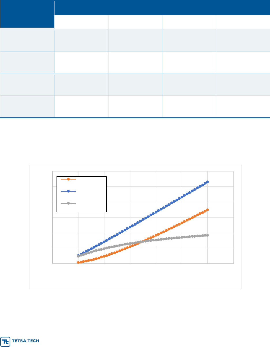
The runoff predicted by the CN method as well as the difference between runoff for developed land and
good condition woods for a given hydrologic soil group and impervious percentage is an exact second-
order polynomial function of P (Figure 2-4). This allows direct calculation of the implications of both
spatial variability and magnitude change in the 1-yr 24-hr event.
Figure 2-4. Curve Number Prediction of Runoff as a Function of Precipitation for Hydrologic Group D
Soils, Developed Land at 80% Imperviousness
Note: Polynomial equation represents the difference between runoff from developed land and runoff from woods in
good condition.
y = -0.0424x
2
+ 0.5531x - 0.0085
0
1
2
3
4
5
6
0 1 2 3 4 5 6 7
Runoff (in)
Precipitation (in)
Woods
Developed
Difference
IDF Project Report September 2020
r 19
3.0 DATA
3.1 NOAA IDF CURVE STATIONS IN MARYLAND
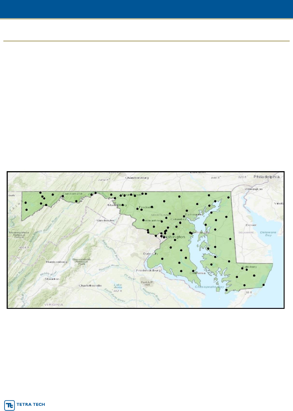
Potential precipitation IDF curves are developed for potential mid-century (ca. 2055) and late-century (ca.
2085) climate scenarios at all 79 Atlas 14 sites within the state of Maryland (Figure 3-1 and Table 3-1). In
addition to the IDF results, we retrieved the AMS series from the NOAA ftp server.
For stations without hourly data, we developed a lookup that identifies the nearest hourly station, which is
used as a surrogate for sub daily precipitation at the station of interest. (Note that the nearest station can
be in an adjoining state.) The results at the surrogate station are then scaled by the average ratio of the
daily total at the station of interest to the total at the surrogate station.
This scaling approach is conceptually similar to that used in Atlas 14 vol, 2, v. 3.0 (Bonnin et al., 2006) to
correct for potential discrepancies between daily totals and the sum of hourly precipitation amounts within
a day. In Atlas 14, the 1-hour through 12-hour duration data are already adjusted by the ratio between
the daily and sum of hourly totals. As the last step of our process applies the estimated change ratio
between historic and future conditions this ratio adjustment procedure does not need to be reapplied
here.
Figure 3-1. NOAA Atlas 14 Sites in Maryland and the District of Columbia

IDF Project Report September 2020
r 20
Table 3-1. Key to NOAA Atlas 14 Sites
18-0185
ANNAPOLIS US NAVAL ACA, MD
18-4780
KEEDYSVILLE, MD
18-0193
ANNAPOLIS POLICE BRKS, MD
18-5080
LA PLATA 1 W, MD
18-0335
ASSATEAGUE IS NATL SEA, MD
18-5111
LAUREL 3 W, MD
18-0465
BALTIMORE WSO ARPT, MD
18-5201
LEONARDTOWN 3 NW, MD
18-0470
BALTIMORE WSO CITY, MD
18-5865
MECHANICSVILLE 5 NE, MD
18-0700
BELTSVILLE, MD
18-5894
MERRILL, MD
18-0705
BELTSVILLE PLANT STN 5, MD
18-5985
MILLINGTON 1 SE, MD
18-0732
BENSON POLICE BARRACKS, MD
18-6350
NATIONAL ARBORETUM DC, MD
18-0915
BLACKWATER REFUGE, MD
18-6408
NEW GERMANY, MD
18-1032
BOYDS 2 NW, MD
18-6620
OAKLAND 1 SE, MD
18-1125
BRIGHTON DAM, MD
18-6770
OWINGS FERRY LANDING, MD
18-1385
CAMBRIDGE WATER TRMT P, MD
18-6844
PARKTON 2 SW, MD
18-1530
CATOCTIN MOUNTAIN PARK, MD
18-6980
PERRY POINT, MD
18-1627
CENTREVILLE, MD
18-7010
PICARDY, MD
18-1710
CHELTENHAM 1 NW, MD
18-7140
POCOMOKE CITY, MD
18-1750
CHESTERTOWN, MD
18-7272
POTOMAC FILTER PLANT, MD
18-1790
CHEWSVILLE-BRIDGEPOR, MD
18-7325
PRINCE FREDERICK 1 N, MD
18-1862
CLARKSVILLE 3 NNE, MD
18-7330
PRINCESS ANNE, MD
18-1890
CLEAR SPRING 1 ENE, MD
18-7700
ROCK HALL, MD
18-1980
COLEMAN 3 WNW, MD
18-7705
ROCKVILLE 1 NE, MD
18-1995
COLLEGE PARK, MD
18-7806
ROYAL OAK 2 SSW, MD
18-2060
CONOWINGO DAM, MD
18-8000
SALISBURY, MD
18-2215
CRISFIELD SOMERS COVE, MD
18-8005
SALISBURY FAA ARPT, MD
18-2282
CUMBERLAND 2, MD
18-8065
SAVAGE RIVER DAM, MD
18-2325
DALECARLIA RESVR DC, MD
18-8315
SINES DEEP CREEK, MD
18-2523
DENTON 2 E, MD
18-8380
SNOW HILL 4 N, MD
18-2700
EASTON POLICE BARRACKS, MD
18-8405
SOLOMONS, MD
18-2770
EDGEMONT, MD
18-8720
TAKOMA PARK BALT AVE, MD
18-2860
ELKTON, MD
18-8855
TONOLOWAY, MD
18-2905
EMMITSBURG, MD
18-8877
TOWSON, MD
18-2906
EMMITSBURG 2 SE, MD
18-9030
UNIONVILLE, MD
18-3230
FORT GEORGE G MEADE, MD
18-9035
U S SOLDIERS HOME DC, MD
18-3348
FREDERICK POLICE BRKS, MD
18-9070
UPPER MARLBORO 3 NNW, MD
18-3355
FREDERICK 3 E, MD
18-9140
VIENNA, MD
18-3415
FROSTBURG 2, MD
18-9409
WESTERNPORT UPRC, MD
18-3675
GLENN DALE BELL STN, MD
18-9440
WESTMINSTER POLICE BRK, MD
18-3795
GRANTSVILLE, MD
18-9570
WILLIAMSPORT, MD
18-3855
GREAT FALLS, MD
18-9750
WOODSTOCK, MD
18-3975
HAGERSTOWN, MD
18-4030
HANCOCK, MD
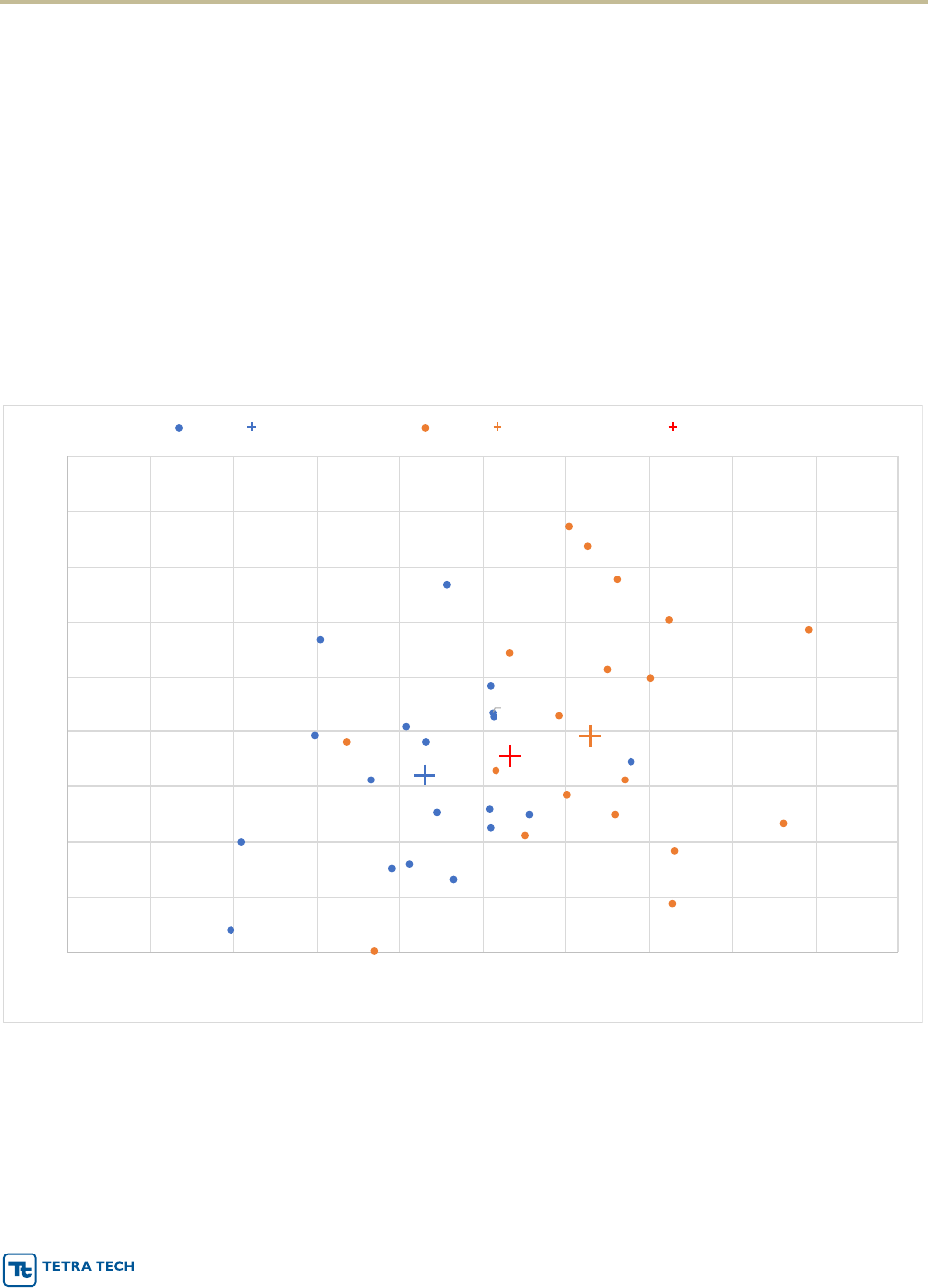
IDF Project Report September 2020
r 21
3.2 CLIMATE MODEL SELECTION
Archives of statistically downscaled climate model output from the 5
th
round Coupled Model
Intercomparison Project (CMIP5) include output from 32 or more Global Climate Models/General
Circulation Models (GCMs) for two or more Representative Concentration Pathways (RCPs) of
greenhouse gas accumulation. While it is possible to estimate IDF curves and 90
th
percentile
precipitation estimates from all GCMs, it is often more useful to identify a smaller set of GCMs that bound
the most likely range of predicted future conditions. Future climate projections are uncertain and are best
used to describe a probability envelope of potential future conditions (an “ensemble of opportunity”) to
which adaptation may be needed. Specifically, climate scenarios that approximate smaller, median, and
larger range of potential changes in precipitation intensity are useful to frame the problem.
Different GCM runs provide differing predictions of future temperature and precipitation. Temperature is
expected to increase under RCP 8.5 versus RCP 4.5 in most locations, but precipitation may increase or
decrease. A typical LASSO biplot of average annual changes in precipitation and temperature from
statistically downscaled GCM runs is shown for Durham, NC in Figure 3-2.
Figure 3-2. Example Biplot of Forecast Changes in Average Annual Precipitation and Air Temperature for
Durham North Carolina for 2050 - 2080 vs. 1950 – 2005
Multiple GCM runs are available from the CMIP5 experiments (approximately 32 GCMs applied to two or
more Representative Concentration Pathway (RCP) greenhouse gas scenarios). We selected
downscaled GCMs from the RCP 4.5 and RCP 8.5 experiments that approximate the 10
th
percentile of
the distribution of predicted change in future rainfall volume, the 90
th
percentile, and the model ensemble
bcc-csm1-1
bcc-csm1-1-m
CanESM2
CCSM4
CNRM-CM5
CSIRO-Mk3-6-0
GFDL-ESM2G
GFDL-ESM2M
HadGEM2-CC365
HadGEM2-ES365
inmcm4
IPSL-CM5A-LR
IPSL-CM5A-MR
IPSL-CM5B-LR
MIROC-ESM
MIROC-ESM-CHEM
MIROC5
MRI-CGCM3
NorESM1-M
bcc-csm1-1-m
CanESM2
CCSM4
CNRM-CM5
CSIRO-Mk3-6-0
GFDL-ESM2G
GFDL-ESM2M
HadGEM2-CC365
HadGEM2-ES365
inmcm4
IPSL-CM5A-LR
IPSL-CM5A-MR
IPSL-CM5B-LR
MIROC-ESM
MIROC-ESM-CHEM
MIROC5
MRI-CGCM3
NorESM1-M
BNU-ESM
0
1
2
3
4
5
6
7
8
9
0 1 2 3 4 5 6 7 8 9 10
CHANGE IN PRECIPITATION (IN/YR)
CHANGE IN TEMPERATURE ( F)
RCP4.5 ensemble mean RCP4.5 RCP8.5 ensemble mean RCP 8.5 overall mean

IDF Project Report September 2020
r 22
median from each of the two RCPs. This approach helps to approximate the potential risk envelope of
future conditions (which are inherently unknowable as they depend on human mitigation actions in the
interim and are also subject to considerable model uncertainty) while rejecting the most extreme outliers
among the population of models. We do not advocate selecting individual GCMs based on their skill in
predicting historic climate for a given area because past performance is not a reliable guide to future
prediction under a changing climate (Dixon et al., 2016).
Because the focus of the work described here is on storm events (whether moderate or extreme),
selection of central and bounding GCM scenarios can be based on the precipitation axis only. For
example, we can select GCM runs from the joint distribution of RCP 4.5 and RCP 8.5 CMIP5 simulations
near the 10
th
, 50
th
, and 90
th
percentiles of the distribution of projected precipitation volume. The analysis
uses the 10
th
and 90
th
percentiles, rather than the most extreme outliers, as it is well recognized that
some individual GCMs may provide unrealistic results for a given area. It is therefore standard practice to
ignore the most extreme outliers and use a model at approximately the 90
th
percentile of the distribution of
a characteristic of interest from the complete set of models as a reasonable upper bound. Use of such an
upper percentile is generally considered appropriate for engineering/hydrologic design planning purposes.
Philip Morefield of U.S. EPA developed Python code for screening climate scenarios as part of the
“Locating and Selecting Scenarios Online” (LASSO) tool that scans the downscaled GCM output archive
monthly data to identify annual and seasonal changes in precipitation volume (lasso.epa.gov). We
adapted code from the LASSO tool to do initial screening for our project on precipitation. However, there
are numerous ways to do this. For instance, one could select based on total annual precipitation volume
or volume in seasons most likely to be associated with floods. Total annual precipitation volume appears
to be a sufficient criterion for extreme event IDF analysis but may not be sufficient for analysis of the 90
th
percentile event. In some cases, GCMs predict that total precipitation volume increase will be largely
confined to the largest events, with longer intervening drought periods, so an increase in total
precipitation volume does not necessarily translate to an increase in the 90
th
percentile event. Therefore,
we ranked scenarios separately relative to the 90
th
percentile event using the following approach:
1. Calculate the sum of rain events that are greater than or equal to the 90
th
percentile historical
rainfall event for each site for each scenario (historical and future).
2. Convert to the large rain event (>=90
th
percentile) depth per day
3. Calculate the relative change rate of the large rain depth per day (rpd): (rpd_gcm-
rpd_hist)/rpd_hist
4. Rank the relative changes from all GCMs and get the 10
th
, RCP4.5 median, RCP85 median, and
90
th
GCMs by value.
This simplified screening procedure does not guarantee that the selected scenarios will always
approximate the 10
th
to 90
th
percentile range, which would require an analysis of all GCMs. It does,
however, help to ensure that a selection of GCMs with relatively different precipitation predictions will be
chosen for more detailed analysis.
Evaluation of downscaled GCM output from the LOCA archive for each MD/DC Atlas 14 station location
yields selections for IDF analysis based on relative change in annual precipitation volume. Table 3-2
shows the 60 LOCA-downscaled GCM and RCP combinations that are evaluated in subsequent tables.
Table 3-3 then shows the selected scenarios for evaluation of mid-century conditions, while Table 3-4
shows results for late-century conditions.
The method selects a wide number of different GCM scenarios but does contain some patterns. For the
90
th
percentile event, the low-end (10
th
percentile of increases) is associated with the lower greenhouse
gas forcing or cooler scenario (RCP 4.5) 70 percent of the time, while the high-end (90
th
percentile) is

IDF Project Report September 2020
r 23
associated with the higher greenhouse gas forcing or warmer scenario (RCP 8.5) 75 percent of the time
for mid-century conditions in Maryland. For late-century conditions, the results are 80 and 53 percent,
respectively. The reduction in the correlation of the wetter scenarios with warmer conditions may result
competing effects of the greater moisture-holding capacity of warmer air versus an increase in the
likelihood of drought.
Systematic differences among GCMs across Maryland are also evident. For instance, for the mid-century
conditions, the 90
th
percentile is represented in 13 out of 60 cases by the MIROC-rcp8.5 scenario, while
the 10
th
percentile is represented in 10 out of 60 cases by the MIROC-ESM_rcp4.5, with no overlap
between the summary statistics for the two GCMs.
Table 3-2. Key to CMIP5 GCM Scenarios in the LOCA Downscaled Climate Data Archive
1
ACCESS1-0_rcp45
21
CSIRO-Mk3-6-0_rcp45
41
HadGEM2-ES_rcp45
2
ACCESS1-0_rcp85
22
CSIRO-Mk3-6-0_rcp85
42
HadGEM2-ES_rcp85
3
ACCESS1-3_rcp45
23
EC-EARTH_rcp45
43
IPSL-CM5A-LR_rcp45
4
ACCESS1-3_rcp85
24
EC-EARTH_rcp85
44
IPSL-CM5A-LR_rcp85
5
bcc-csm1-1-m_rcp45
25
FGOALS-g2_rcp45
45
IPSL-CM5A-MR_rcp45
6
bcc-csm1-1-m_rcp85
26
FGOALS-g2_rcp85
46
IPSL-CM5A-MR_rcp85
7
CanESM2_rcp45
27
GFDL-CM3_rcp45
47
MIROC5_rcp45
8
CanESM2_rcp85
28
GFDL-CM3_rcp85
48
MIROC5_rcp85
9
CCSM4_rcp45
29
GFDL-ESM2G_rcp45
49
MIROC-ESM_rcp45
10
CCSM4_rcp85
30
GFDL-ESM2G_rcp85
50
MIROC-ESM_rcp85
11
CESM1-BGC_rcp45
31
GFDL-ESM2M_rcp45
51
MIROC-ESM-CHEM_rcp45
12
CESM1-BGC_rcp85
32
GFDL-ESM2M_rcp85
52
MIROC-ESM-CHEM_rcp85
13
CESM1-CAM5_rcp45
33
GISS-E2-H_rcp45
53
MPI-ESM-LR_rcp45
14
CESM1-CAM5_rcp85
34
GISS-E2-H_rcp85
54
MPI-ESM-LR_rcp85
15
CMCC-CM_rcp45
35
GISS-E2-R_rcp45
55
MPI-ESM-MR_rcp45
16
CMCC-CM_rcp85
36
GISS-E2-R_rcp85
56
MPI-ESM-MR_rcp85
17
CMCC-CMS_rcp45
37
HadGEM2-AO_rcp45
57
MRI-CGCM3_rcp45
18
CMCC-CMS_rcp85
38
HadGEM2-AO_rcp85
58
MRI-CGCM3_rcp85
19
CNRM-CM5_rcp45
39
HadGEM2-CC_rcp45
59
NorESM1-M_rcp45
20
CNRM-CM5_rcp85
40
HadGEM2-CC_rcp85
60
NorESM1-M_rcp85

IDF Project Report September 2020
r 24
Table 3-3. Bounding Scenarios for Analysis of Changes in Precipitation Volume, ca. 2056
Site
10
th
Percentile
RCP4.5 Median
RCP8.5 Median
90
th
percentile
18-0015
50
5
30
60
18-0185
49
3
14
52
18-0193
17
3
14
32
18-0335
15
3
2
34
18-0465
49
23
4
32
18-0470
43
41
4
19
18-0700
40
23
16
11
18-0705
49
39
16
11
18-0732
44
23
14
34
18-0915
45
13
4
48
18-1032
37
1
20
9
18-1125
57
51
20
9
18-1385
17
13
30
60
18-1530
29
59
36
12
18-1627
40
3
38
48
18-1710
57
39
16
60
18-1750
58
23
4
10
18-1790
35
53
22
18
18-1862
57
55
22
11
18-1890
44
1
8
11
18-1980
17
13
38
56
18-1995
57
41
24
11
18-2060
58
7
30
20
18-2215
49
19
2
11
18-2282
29
7
58
48
18-2325
43
39
24
60
18-2523
49
39
46
56
18-2700
50
33
6
32
18-2770
29
3
20
12
18-2860
49
51
16
6

IDF Project Report September 2020
r 25
Site
10
th
Percentile
RCP4.5 Median
RCP8.5 Median
90
th
percentile
18-2905
50
25
20
48
18-2906
50
25
4
48
18-3230
40
23
20
60
18-3348
35
1
36
9
18-3355
35
1
16
18
18-3415
45
7
8
14
18-3675
44
1
24
48
18-3795
43
51
36
34
18-3855
40
3
16
47
18-3975
35
7
22
48
18-4030
37
39
8
52
18-4780
29
1
8
48
18-5080
17
19
4
60
18-5111
54
15
56
60
18-5201
45
3
4
48
18-5865
44
39
8
32
18-5894
29
15
12
34
18-5985
40
13
30
56
18-6350
57
3
18
10
18-6408
2
3
8
14
18-6620
37
11
12
47
18-6770
57
7
24
48
18-6844
58
15
2
48
18-6980
29
1
22
60
18-7010
45
25
58
32
18-7140
17
31
30
21
18-7272
40
53
24
6
18-7325
44
55
4
9
18-7330
38
3
12
36
18-7700
17
23
2
56
18-7705
57
35
8
11

IDF Project Report September 2020
r 26
Site
10
th
Percentile
RCP4.5 Median
RCP8.5 Median
90
th
percentile
18-7806
57
15
46
22
18-8000
20
29
36
41
18-8005
38
7
2
34
18-8065
17
3
36
18
18-8315
37
39
12
34
18-8380
49
39
2
34
18-8405
45
25
6
48
18-8720
17
39
24
10
18-8855
37
51
58
60
18-8877
49
1
24
6
18-9030
49
13
22
32
18-9035
17
33
20
10
18-9070
37
3
18
21
18-9140
45
7
46
11
18-9409
1
3
8
32
18-9440
49
41
8
48
18-9570
44
7
10
11
18-9750
57
1
16
9
See Table 3-1 for site indices; Table 3-2 for identification of GCM scenarios.

IDF Project Report September 2020
r 27
Table 3-4. Bounding Scenarios for Analysis of Changes in Precipitation Volume, ca. 2085
Site
10
th
Percentile
RCP4.5 Median
RCP8.5 Median
90
th
percentile
18-0015
5
29
16
60
18-0185
43
15
52
22
18-0193
43
15
24
22
18-0335
16
33
6
58
18-0465
17
31
48
34
18-0470
49
33
58
18
18-0700
41
7
6
60
18-0705
5
29
6
60
18-0732
41
1
6
34
18-0915
41
55
46
11
18-1032
41
23
40
11
18-1125
37
1
32
11
18-1385
37
23
40
21
18-1530
44
1
16
11
18-1627
37
55
24
22
18-1710
41
3
24
60
18-1750
57
15
42
34
18-1790
17
1
32
11
18-1862
41
19
16
11
18-1890
41
53
10
21
18-1980
44
53
48
56
18-1995
5
15
6
11
18-2060
49
53
6
11
18-2215
25
1
60
24
18-2282
44
7
6
27
18-2325
43
1
36
11
18-2523
17
53
36
22
18-2700
5
3
36
21
18-2770
5
1
6
34
18-2860
37
15
20
40

IDF Project Report September 2020
r 28
Site
10
th
Percentile
RCP4.5 Median
RCP8.5 Median
90
th
percentile
18-2905
25
55
32
11
18-2906
17
1
40
11
18-3230
44
59
32
60
18-3348
5
59
32
21
18-3355
2
15
16
56
18-3415
38
35
10
33
18-3675
44
33
6
22
18-3795
43
7
6
21
18-3855
43
15
24
34
18-3975
39
9
32
11
18-4030
57
9
16
33
18-4780
41
53
8
21
18-5080
43
15
18
10
18-5111
41
1
36
56
18-5201
44
3
40
11
18-5865
44
3
48
10
18-5894
43
57
16
4
18-5985
37
23
32
34
18-6350
5
7
18
11
18-6408
43
19
8
21
18-6620
5
19
8
56
18-6770
41
31
24
27
18-6844
37
39
14
11
18-6980
44
29
16
60
18-7010
44
19
8
21
18-7140
19
59
42
11
18-7272
5
49
6
11
18-7325
41
7
40
11
18-7330
17
23
36
4
18-7700
43
31
48
54
18-7705
44
3
32
10

IDF Project Report September 2020
r 29
Site
10
th
Percentile
RCP4.5 Median
RCP8.5 Median
90
th
percentile
18-7806
5
9
24
56
18-8000
25
55
6
14
18-8005
5
57
10
4
18-8065
25
7
10
33
18-8315
39
19
14
6
18-8380
8
31
6
47
18-8405
44
23
24
22
18-8720
57
1
32
11
18-8855
43
9
8
34
18-8877
44
53
36
34
18-9030
5
13
52
22
18-9035
57
15
52
11
18-9070
43
29
6
56
18-9140
41
31
36
54
18-9409
43
7
10
4
18-9440
41
19
20
11
18-9570
41
55
32
21
18-9750
49
13
16
21
See Table 3-1 for site indices; Table 3-2 for identification of GCM scenarios.
GCM scenarios for the analysis of changes in the 90
th
percentile 24-hour precipitation event were
screened on the basis of percentage of events greater than the historic 90
th
percentile event. The
selected bounding scenarios are summarized in Table 3-5 (for ca. 2055 conditions based on 2040-2069
GCM output) and in Table 3-6 (for ca. 2085 conditions based on 2070-2099 GCM output). Identities of
the GCM scenarios are shown in Table 3-2.
For the 90
th
percentile event, the low-end (10
th
percentile of increases) is associated with the lower
greenhouse gas forcing scenario (RCP 4.5) 71 percent of the time, while the high-end (90
th
percentile) is
associated with the higher greenhouse gas forcing scenario (RCP 8.5) 68 percent of the time for ca. 2056
conditions across Maryland. For ca. 2085 predictions, the results are 82 and 94 percent, respectively.

IDF Project Report September 2020
r 30
Table 3-5. Bounding Scenarios for Analysis of the 90
th
Percentile 24-hour Precipitation Event, ca. 2056
Site
10
th
Percentile
RCP4.5 Median
RCP8.5 Median
90
th
percentile
18-0015
49
35
4
48
18-0185
14
9
28
15
18-0193
29
9
12
15
18-0335
45
21
32
56
18-0465
29
55
40
52
18-0470
14
23
10
48
18-0700
33
19
56
22
18-0705
33
55
10
16
18-0732
13
59
20
38
18-0915
9
31
24
22
18-1032
59
41
12
36
18-1125
26
5
20
38
18-1385
6
7
10
39
18-1530
8
31
18
56
18-1627
17
1
30
34
18-1710
7
3
46
21
18-1750
29
7
6
39
18-1790
13
7
32
21
18-1862
50
19
2
21
18-1890
8
19
32
11
18-1980
45
9
18
40
18-1995
26
51
18
48
18-2060
55
33
30
19
18-2215
60
15
34
54
18-2282
29
13
14
48
18-2325
45
1
20
22
18-2523
45
31
46
48
18-2700
59
7
38
22
18-2770
45
13
20
38
18-2860
17
51
4
22

IDF Project Report September 2020
r 31
Site
10
th
Percentile
RCP4.5 Median
RCP8.5 Median
90
th
percentile
18-2905
49
25
48
28
18-2906
49
25
46
18
18-3230
29
59
4
56
18-3348
57
29
22
40
18-3355
26
59
10
21
18-3415
57
19
10
21
18-3675
7
53
2
10
18-3795
29
45
12
52
18-3855
35
3
2
47
18-3975
57
41
10
28
18-4030
23
39
2
56
18-4780
23
41
2
40
18-5080
7
9
28
56
18-5111
49
19
2
21
18-5201
17
29
24
39
18-5865
14
25
18
38
18-5894
17
3
10
27
18-5985
50
1
32
46
18-6350
26
1
4
15
18-6408
8
45
10
60
18-6620
50
37
4
27
18-6770
33
55
46
39
18-6844
33
5
18
27
18-6980
7
43
18
40
18-7010
26
41
14
27
18-7140
19
59
32
54
18-7272
14
57
2
38
18-7325
43
37
18
22
18-7330
9
1
52
56
18-7700
29
3
6
39
18-7705
44
59
24
36

IDF Project Report September 2020
r 32
Site
10
th
Percentile
RCP4.5 Median
RCP8.5 Median
90
th
percentile
18-7806
49
9
30
21
18-8000
45
17
8
28
18-8005
29
17
24
56
18-8065
43
37
22
18
18-8315
51
39
36
60
18-8380
19
3
4
34
18-8405
57
1
10
36
18-8720
50
55
18
15
18-8855
45
33
2
36
18-8877
33
3
4
36
18-9030
59
9
12
21
18-9035
33
1
46
22
18-9070
54
37
44
38
18-9140
17
51
28
21
18-9409
5
23
40
32
18-9440
50
43
48
28
18-9570
26
41
18
40
18-9750
8
51
48
56
See Table 3-1 for site indices; Table 3-2 for identification of GCM scenarios.

IDF Project Report September 2020
r 33
Table 3-6. Bounding Scenarios for Analysis of the 90
th
Percentile 24-hour Precipitation Event, ca. 2085
Site
10
th
Percentile
RCP4.5 Median
RCP8.5 Median
90
th
percentile
18-0015
17
33
52
16
18-0185
17
55
2
42
18-0193
19
33
2
56
18-0335
9
13
32
12
18-0465
57
47
24
12
18-0470
14
19
52
36
18-0700
13
23
60
58
18-0705
17
23
36
12
18-0732
17
53
52
16
18-0915
5
33
52
42
18-1032
43
19
2
15
18-1125
57
31
36
18
18-1385
5
33
2
54
18-1530
19
23
10
48
18-1627
5
11
36
12
18-1710
19
55
18
54
18-1750
5
33
18
12
18-1790
14
53
18
12
18-1862
8
23
2
22
18-1890
19
7
42
22
18-1980
25
23
58
22
18-1995
13
5
28
56
18-2060
17
19
6
28
18-2215
60
39
18
46
18-2282
29
53
42
28
18-2325
49
9
52
54
18-2523
25
29
36
16
18-2700
25
11
58
4
18-2770
29
55
6
46
18-2860
47
33
24
3

IDF Project Report September 2020
r 34
Site
10
th
Percentile
RCP4.5 Median
RCP8.5 Median
90
th
percentile
18-2905
19
7
18
56
18-2906
19
31
58
12
18-3230
43
39
24
42
18-3348
43
35
18
22
18-3355
26
31
18
54
18-3415
7
35
16
6
18-3675
14
29
6
16
18-3795
7
59
60
22
18-3855
25
27
2
34
18-3975
31
9
18
12
18-4030
39
53
28
52
18-4780
59
39
6
40
18-5080
17
23
32
12
18-5111
13
9
12
40
18-5201
7
5
18
56
18-5865
17
31
18
54
18-5894
7
1
40
54
18-5985
25
27
10
56
18-6350
25
5
18
21
18-6408
19
37
40
6
18-6620
7
9
30
16
18-6770
17
29
18
16
18-6844
59
33
24
12
18-6980
47
33
2
22
18-7010
29
23
42
34
18-7140
26
51
4
46
18-7272
57
37
12
15
18-7325
17
51
36
16
18-7330
44
13
32
46
18-7700
8
23
2
22
18-7705
13
33
24
48

IDF Project Report September 2020
r 35
Site
10
th
Percentile
RCP4.5 Median
RCP8.5 Median
90
th
percentile
18-7806
25
11
10
4
18-8000
31
15
18
48
18-8005
9
15
18
34
18-8065
29
37
58
4
18-8315
26
13
30
4
18-8380
25
1
4
45
18-8405
59
31
28
34
18-8720
43
23
58
16
18-8855
59
13
6
54
18-8877
5
39
6
4
18-9030
25
29
54
56
18-9035
26
29
60
16
18-9070
25
9
36
12
18-9140
30
47
12
56
18-9409
7
53
36
46
18-9440
26
23
10
16
18-9570
19
23
6
40
18-9750
8
47
52
54
See Table 3-1 for site indices; Table 3-2 for identification of GCM scenarios.

IDF Project Report September 2020
r 36
(This page left intentionally blank.)

IDF Project Report September 2020
r 37
4.0 RESULTS – EXTREME PRECIPITATION
The methods described in Section 2.1 were applied to the four GCMs selected for each of two future time
periods and the historic time period at the 79 Maryland Atlas 14 stations (Section 3.0). Results are
provided electronically in two databases, one for the IDF analysis and one for the peaks-over-threshold
analysis of the 90
th
percentile 24-hour event. The two databases (IDF-db.xlsx and 90
th
%le-db.xlsx) are
provided in Microsoft Excel™ format. Each database contains three tabs.
The results of the analyses are contained on the IDFdb tab. For each station, time horizon, and GCM
combination, the IDFdb tab in the 90
th
%le-db.xlsx database provides a single result (the estimated 24-
hour 90
th
percentile event). The IDFdb tab in the IDF-db.xlsx database provides, for each station, time
horizon, and GCM combination, sets of 10 durations (5-minute to 24-hour) for 10 difference recurrence
intervals.
To aid the user in exploring the databases, each contains a Graph tab for visualization. On this tab, the
user can select a station from a drop-down list. For the IDF-db, the user can also select a recurrence
interval. The workbook will then retrieve the requested data and display it in both tabular and graphical
form (see examples below).
Results of the IDF analysis suggest a widespread risk of increase under future conditions in Maryland for
the intensity of extreme precipitation events of a given duration and recurrence. However, this increase is
not consistent among GCM scenarios downscaled by LOCA. At many stations, the future results suggest
more of an increase in the cone of uncertainty than a unimodal increase in intensity – implying a risk of
more intense events, but not always a consensus. For some GCM simulations the predicted intensity of
low recurrence events decreases, presumably due to drier conditions predicted during the convective
storm season. The method also assumes that relative bias between historical LOCA-downscaled GCM
performance and observed data will be retained into the future – which in some cases where the fit to
historic conditions is poor can lead to extreme future predictions that may not be physically realistic. It
does appear that LOCA fails to provide a strong match to the distribution of historic high precipitation
events, especially for stations near the land-water interface, even though the developers claim that
“LOCA produces better estimates of extreme days” (Pierce et al., 2014). A newly released pre-print of
Wang et al. (2020) appears to show that LOCA tends to under-estimate the magnitude of extreme
precipitation events due to the way in which the historic training data set was constructed.
We also noted that the selection of GCMs that have higher or lower total annual precipitation volume
often does not guarantee a similar alteration in the intensity of low-recurrence storm events. This could
be associated with GCMs that predict a higher frequency of moderate intensity events and/or a seasonal
shift away from the convective storm season.
A careful look at the results reveals instances where projected results for a given GCM do not increase
monotonically across recurrence interval – especially for events with greater than 100-yr recurrence
intervals. These anomalies occur due to the statistical nature of the analysis and the last step of the
analysis in which the projected results are renormalized against the published IDF curve ordinates. This
can result in some crossing behavior if the shape of the relationship between intensity and recurrence
interval for a given duration is substantially different between historical AMS data and the GCM output
and is exacerbated where results are extrapolated beyond the 30-yr time window for future climate output
(e.g., predicting change in a 500-year event from statistical fit to a 30-year sample). These small
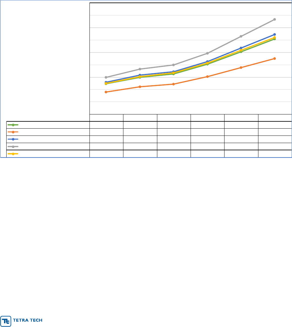
IDF Project Report September 2020
r 38
discrepancies should not interfere with the intended use of the results to investigate the potential range of
risk for which adaptation may be required under further climate.
The predicted intensity of the 90
th
percentile 24-hour event does not show a consistent increase at most
stations under future conditions. This is in line with studies that suggest total annual precipitation volume
will most likely increase under future climate, but that much of this increase will be associated with more
extreme, low-recurrence events (Easterling et al., 2017). The 90
th
percentile results thus appear to be
“good news” as they suggest that many water quality BMPs that are optimized to capture and treat
pollutants associated with sub-yearly recurrence events are likely to continue to provide expected
services under future climate.
Representative figures from the reporting databases are shown in Figure 4-1 through Figure 4-3.
Figure 4-1. Projected 25-year IDF Curves for Baltimore WSO Airport ca. 2055
1-hr 2-hr 3-hr 6-hr 12-hr 24-hr
Historic - Atlas14
2.46 3.00 3.27 4.05 5.06 6.08
2055-10th - MIROC-ESM_rcp45
1.80 2.23 2.43 3.06 3.78 4.51
2055-RCP4.5-50th - EC-EARTH_rcp45
2.58 3.16 3.44 4.26 5.35 6.46
2055-RCP8.5-50th - ACCESS1-3_rcp85
2.97 3.65 3.99 4.94 6.28 7.66
2055-90th - GFDL-ESM2M_rcp85
2.51 3.06 3.34 4.13 5.17 6.22
0
1
2
3
4
5
6
7
8
9
Rainfall (inch)
Rainfall Duration
BALTIMORE WSO ARPT, MD (18-0465), 25-year Recurrence, ca. 2055

IDF Project Report September 2020
r 39
Figure 4-2. Projected 25-year IDF Curves for Baltimore WSO Airport ca. 2085
1-hr 2-hr 3-hr 6-hr 12-hr 24-hr
Historic - Atlas14
2.46 3.00 3.27 4.05 5.06 6.08
2085-10th - CMCC-CMS_rcp45
2.66 3.24 3.54 4.37 5.49 6.63
2085-RCP4.5-50th - GFDL-ESM2M_rcp45
2.60 3.18 3.47 4.30 5.41 6.53
2085-RCP8.5-50th - MIROC5_rcp85
2.70 3.31 3.62 4.49 5.69 6.90
2085-90th - GISS-E2-H_rcp85
3.55 4.43 4.87 6.07 7.94 9.90
0
1
2
3
4
5
6
7
8
9
10
11
Rainfall (inch)
Rainfall Duration
BALTIMORE WSO ARPT, MD (18-0465), 25-year Recurrence, ca. 2085

IDF Project Report September 2020
r 40
Figure 4-3. Projected Results for 90
th
Percentile 24-hour Precipitation Event, Aberdeen-Phillips Field
For analysis of the 90th percentile 24 hr event, the 10th percentile (low), median,
and 90th percentile (high) GCM categories are based on relative projected change
in total precipitation volume above the historical 90th-percentile 24-hr event. This
approach does not guarantee that the change in magnitude of the estimated
90th-percentile 24-hr events will scale in the same order as the low, median, and
high impact GCMs as the change in volume may be focused in more extreme,
low-recurrence events; however, it does ensure that the selected GCMs span a
range of different projected characteristics for future climate conditions.
Future climate projections are based on 30-year periods centered at 2055 and 2085.
Historic
2055-
10th
2055-
RCP4.5-
50th
2055-
RCP8.5-
50th
2055-
90th
2085-
10th
2085-
RCP4.5-
50th
2085-
RCP8.5-
50th
2085-
90th
Inches/dy
0.872 0.840 0.824 0.823 0.867 0.857 0.766 0.935 0.967
0.000
0.200
0.400
0.600
0.800
1.000
1.200
Depth (in/day)
90th Percentile 24-hr Event, ABERDEEN PHILLIPS FLD,
MD (18-0015)

IDF Project Report September 2020
r 41
5.0 RESULTS – EVENT RUNOFF AND BMP SIMULATIONS
The SWMM simulations are performed at all 79 Atlas 14 stations in Maryland. Each station is evaluated
for two future periods centered at 2055 and 2085). For each time period, results are generated for four
GCMs representing the 10
th
, median RCP 4.5, median RCP 8.5, and 90
th
percentile in terms of predicted
change in future total precipitation volume. Simulations are run for the 1, 2, 10, and 100-yr 24-hour storm
events, plus the 90
th
percentile 24-hour event. The two BMPs are simulated with three levels of
imperviousness (25%, 50%, and 80%). This provides a database of 20,574 simulations.
Because of the large number of runs completed, results are provided in four separate electronic
databases:
• SWMM_BIORETENTION_IDF_OUTPUT_SUMMARY.xlsx
• SWMM_BIORETENTION_POT_OUTPUT_SUMMARY.xlsx
• SWMM_WETPOND_IDF_OUTPUT_SUMMARY.xlsx
• SWMM_WETPOND_POT_OUTPUT_SUMMARY.xlsx
Within each database, the first tab provides the raw results from each individual simulation. These are
results for a 48-hour simulation (with storm event on the first day) for a drainage area (nominal 1 acre for
bioretention and 25-acre for extended wet detention). Results are generated as total runoff in cubic feet
(per two days) with peak flow in cfs. The second tab contains summaries of the first tab at varying levels
of aggregation.
5.1 RUNOFF
SWMM5 simulated runoff prior to entering the BMP is equivalent to the unmanaged runoff from the site
and can be used to build intensity-frequency relationships for future runoff events. The frequency is the
same as the frequency of the underlying rain event. Summary results for the 1-acre bioretention
simulation produce estimates of peak flow as cfs/ac as well as estimates for total storm flow. Results for
peak flow (averaged across all sites) are shown in Figure 5-1, separated by recurrence interval and
impervious percentage. By the end of the century, peak runoff rates are predicted to increase, on
average, about 13 – 14 percent, with slightly higher increases for longer recurrence intervals and lower
impervious percentages.

IDF Project Report September 2020
r 42
Figure 5-1. Historic and Future Peak Flow Averages by Recurrence
5.2 BIORETENTION BMP
Raw output for the bioretention simulations is displayed in the following format. Columns A through I
provide the run identification information, such as the following:
SWMM Output------------------------------------------------------------------------------------------------------------------------------------------
StationName
StationID
Year
GCM_RCP
BMP_Type
ANALYSIS_Type
WQ_Depth
EVENT_Type
P_IMPERV
ABERDEEN PHILLIPS FLD, MD
18-0015
Historic
Atlas14
Bioretention
IDF
2.67
1-yr 24-hr
25
Here, “Year” can be Historic, 2055, or 2085 and “GCM_RCP” can be either Atlas 14 or the name of a
future climate GCM. “ANALYSIS_Type” is either IDF or POT, where POT represents the 90
th
percentile
analysis. “WQ_Depth” is the design requirement water quality depth in inches, and “P_Imper” is
impervious percentage. The other variables are self-explanatory.
Columns J through M provide the SWMM hydraulic output. The volumes are totals over the 48-hour
simulation period:
PeakFlow_cfs
Overflow_cf
Underdrain_outflow_cf
TotalOutflow
2.10
3,792
1,820
5,612
Finally, columns O through R summarize the change relative to Atlas 14 (historic) design conditions:
Change --------------------------------------------
PeakFlow_cfs%
Overflow_cf%
Underdrain_outflow_cf%
TotalOutflow%
12.05%
16.65%
3.77%
12.47%
0
2
4
6
8
10
12
14
2000 2020 2040 2060 2080 2100
Peak Runoff (cfs/ac)
80% Imp 50% Imp 25% Imp
100yr
10yr
2yr

IDF Project Report September 2020
r 43
Bioretention cells are designed to provide water quality treatment for the 90
th
percentile 24-hour rainfall
event. We noted in Section 4.0 that the 90
th
percentile event under future climate conditions was
frequently predicted to be smaller than historic, with overall increases in total precipitation volume
concentrated in more extreme events. This is borne out in the analysis of bioretention response to this
event (the “POT” database). Taking the average of the median change across all sites, the peak flow and
total outflow decline by -17 and -18%, respectively, for 2055, and by -11 and -12% for 2085 (Table 5-1.
On average, bioretention produces no bypass overflow under historic or future conditions for the 90
th
-
percentile event. There is, however, a wide range in predicted responses between sites and an even
larger range between individual site and climate scenario combinations.
Table 5-1. Summary of Response of Bioretention to 90
th
-percentile Event
Average of median change across all sites
Peak Flow (cfs)
Overflow (ft
3
)
Underdrain (ft
3
)
Total Outflow (ft
3
)
2055
-17.26%
0%
-18.02%
-18.02%
2085
-11.33%
0%
-11.93%
-11.93%
Range of median change over sites
2055
-57.10% to 12.29%
0%
-58.57% to 18.91%
-58.57% to 18.91%
2085
-50.48% to 13.56%
0%
-51.49% to 15.56%
-51.49% to 15.56%
Range over all individual scenarios
2055
-75.69% to 392.4%
0% to 21.44%
-79.00% to 87.80%
-79.00% to 101.8%
2085
-73.35% to 1724%
0% to 82.41%
-76.29% to 110.5%
-76.29% to 141.7%
Median change versus impervious %
I=25
-17.72%
0%
-21.42%
-21.42%
I=50
-15.14%
0%
-16.32%
-16.32%
I=80
-12.05%
0%
-12.51%
-12.51%
Bioretention is not designed to fully treat larger low-recurrence events with longer return periods.
Averaging over the medians of all sites and future scenarios (incorporating 1-year through 100-year 24-
hour events) the peak flow, bypass (overflow), and total outflow increase by 8, 11, and 7%, respectively
for 2055 and by 16, 21, and 14% by 2085.

IDF Project Report September 2020
r 44
Table 5-2. Summary of Responses of Bioretention to Future 1-year through 100-year Events
Average of median change across all sites
Peak Flow (cfs)
Overflow (ft
3
)
Underdrain (ft
3
)
Total Outflow (ft
3
)
2055
8.43%
11.13%
1.73%
7.30%
2085
15.71%
20.76%
2.97%
13.54%
Range of median change over sites
2055
-1.29% to 22.31%
-1.44% to 29.56%
-0.20% to 4.24%
-1.23% to 20.65%
2085
2.31% to 34.65%
3.58% to 42.29%
0.44% to 6.45%
1.96% to 27.30%
Range over all individual scenarios
2055
-48.28% to 201.0%
-58.59% to 264.7%
-10.72% to 12.68%
-48.35% to 228.6%
2085
-43.36% to 139.4%
-52.48% to 173.8%
-10.66% to 12.02%
-44.96% to 151.1%
Median change versus impervious %
I=25
10.51%
12.75%
2.21%
10.13%
I=50
11.15%
15.33%
2.23%
9.73%
I=80
12.87%
18.87%
2.32%
9.46%
The bioretention results for outflows by different pathways for all scenarios in all areas of Maryland are
summarized graphically in Figure 5-2 and Figure 5-3. The left side of these figures shows the low-range
responses (based on the 90
th
-percentile event simulations) while the right side shows the high-range
responses (based on the IDF simulations) at varying levels of imperviousness. Results for the 25%
impervious case look somewhat anomalous because the Simple Method sizing rule tends to undersize
bioretention when imperviousness is low. For larger, low-recurrence events, the bioretention response
becomes approximately linear.
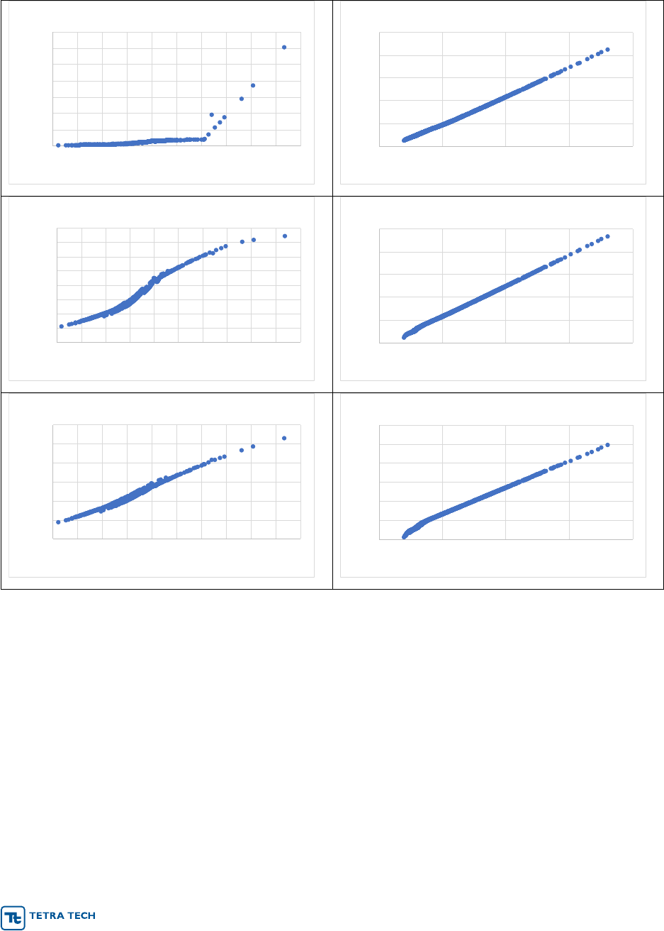
IDF Project Report September 2020
r 45
Figure 5-2. Bioretention Simulation Results for Peak Outflow as a Function of Total Storm Depth
Note: Figures on left side show closeup of responses to higher frequency, lower volume peak events; figures on right side show
responses to lower frequency extreme events.
0
0.05
0.1
0.15
0.2
0.25
0.3
0.35
0.5 0.6 0.7 0.8 0.9 1 1.1 1.2 1.3 1.4 1.5
Peak Flow (cfs)
Storm Depth (in)
Bioretention Site Peak Flow at 25% imperv
0
5
10
15
20
25
0 5 10 15 20
Peak Flow (cfs)
Storm Depth (in)
Bioretention Site Peak Flow at 25% imperv
0
0.005
0.01
0.015
0.02
0.025
0.03
0.035
0.04
0.5 0.6 0.7 0.8 0.9 1 1.1 1.2 1.3 1.4 1.5
Peak Flow (cfs)
Storm Depth (in)
Bioretention Site Peak Flow at 50% imperv
0
5
10
15
20
25
0 5 10 15 20
Peak Flow (cfs)
Storm Depth (in)
Bioretention Site Peak Flow at 50% imperv
0
0.01
0.02
0.03
0.04
0.05
0.06
0.5 0.6 0.7 0.8 0.9 1 1.1 1.2 1.3 1.4 1.5
Peak Flow (cfs)
Storm Depth (in)
Bioretention Site Peak Flow at 80% imperv
0
5
10
15
20
25
30
0 5 10 15 20
Peak Flow (cfs)
Storm Depth (in)
Bioretention Site Peak Flow at 80% imperv
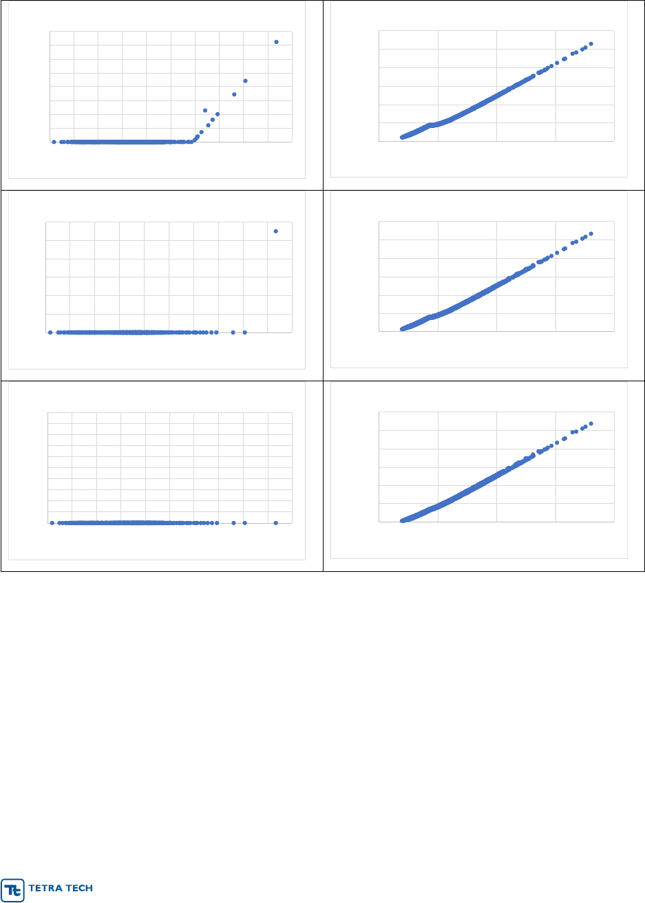
IDF Project Report September 2020
r 46
Figure 5-3. Bioretention Simulation Results for Overflow Volume as a Function of Total Storm Depth
Note: Figures on left side show closeup of responses to higher frequency, lower volume peak events; figures on right side show
responses to lower frequency extreme events.
0
100
200
300
400
500
600
700
800
0.5 0.6 0.7 0.8 0.9 1 1.1 1.2 1.3 1.4 1.5
Outflow Volume (cf)
Storm Depth (in)
Bioretention Overflow Volume at 25% imperv
0
10000
20000
30000
40000
50000
60000
0 5 10 15 20
Outflow Volume (cf)
Storm Depth (in)
Bioretention Overflow Volume at 25% imperv
0
10
20
30
40
50
60
0.5 0.6 0.7 0.8 0.9 1 1.1 1.2 1.3 1.4 1.5
Outflow Volume (cf)
Storm Depth (in)
Bioretention Overflow Volume at 50% imperv
0
10000
20000
30000
40000
50000
60000
0 5 10 15 20
Outflow Volume (cf)
Storm Depth (in)
Bioretention Overflow Volume at 50% imperv
0
0.1
0.2
0.3
0.4
0.5
0.6
0.7
0.8
0.9
1
0.5 0.6 0.7 0.8 0.9 1 1.1 1.2 1.3 1.4 1.5
Outflow Volume (cf)
Storm Depth (in)
Bioretention Overflow Volume at 80% imperv
0
10000
20000
30000
40000
50000
60000
0 5 10 15 20
Outflow Volume (cf)
Storm Depth (in)
Bioretention Overflow Volume at 80% imperv

IDF Project Report September 2020
r 47
5.3 EXTENDED WET DETENTION BMP
Raw output for the extended wet detention simulations is displayed a format similar to bioretention.
Columns A through J provide the run identification information. This differs from bioretention in adding
the scenario rainfall (column H) and the channel protection volume stage for the design (column J).
Columns K through M provide the SWMM hydraulic output. “Site_peak_flow_cfs” is the instantaneous
peak output from the BMP, including both the from the orifice and flow over the weir. “Site_volume_cf” is
the total outflow from the wet pond (in cubic feet) over the 48-hour simulation period. For this BMP,
“TotalOutflow” is the same as Site_volume_cf but is included for consistency with the bioretention output
format.
Site_peak_flow_cfs
Site_volume_cf
TotalOutflow
30.952
147,229
147,229
Finally, columns O and R summarize the change relative to Atlas 14 (historic) design conditions:
PeakFlow_cfs%
TotalOutflow%
11.31%
12.17%
As was noted for bioretention, the 90
th
percentile event under future climate conditions was frequently
predicted to be smaller than historic, with overall increases in total precipitation volume concentrated in
more extreme events. Accordingly, the wet pond simulations also tend to show a decline in outflow for
the 90
th
percentile event, but with substantial variability among scenarios (Table 5-3). Peak flow is
relatively insensitive to impervious percentage for the 90
th
-percentile event as releases from the pond are
controlled by the orifice.
Table 5-3. Summary of Response of Extended Wet Detention to 90
th
-percentile Event
Average of median change across all sites
Peak Flow
Total Outflow
2055
-5.97%
-10.70%
2085
-3.95%
-7.06%
Range of median change over sites
2055
-20.74% to 5.36%
-36.15% to 10.96%
2085
-18.10% to 4.82%
-31.83% to 9.35%
Range over all individual scenarios
2055
-30.13% to 33.88%
-51.27% to 72.73%
2085
-28.15% to 44.88%
-48.82% to 111.09%
Median change versus impervious %
25
-6.81%
-12.26%
50
-5.09%
-9.19%
80
-3.94%
-7.15%

IDF Project Report September 2020
r 48
For larger low recurrence events, averaging over the medians of all sites and future scenarios
(incorporating 1-year through 100-year 24-hour events) the peak flow and total outflow increase by 22
and 7%, respectively for 2055 and by 41 and 13% by 2085 for extended wet detention (Table 5-4).
Table 5-4. Summary of Responses of Extended Wet Detention to Future 1-year through 100-year Events
Average of median change across all sites
Peak Flow
Total Outflow
2055
21.89%
6.89%
2085
41.44%
12.81%
Range of median change over sites
2055
-1.84% to 58.99%
-1.23% to 20.17%
2085
6.21% to 108.62%
1.93% to 25.58%
Range over all individual scenarios
2055
-75.39% to 607.22%
-48.65% to 232.77%
2085
-70.79% to 778.38%
-45.28% to 152.61%
Median change versus impervious %
25
28.15%
10.13%
50
32.26%
9.20%
80
27.08%
8.61%
The extended wet detention basin results for all scenarios in all areas of Maryland are summarized
graphically in Figure 5-4 and Figure 5-5. The left side of these figures shows the low-range responses
(based on the 90
th
-percentile event simulations) while the right side shows the high-range responses
(based on the IDF simulations) at varying levels of imperviousness. The separate lines in the peak flow
responses reflect the differing design criteria in eastern and western Maryland.
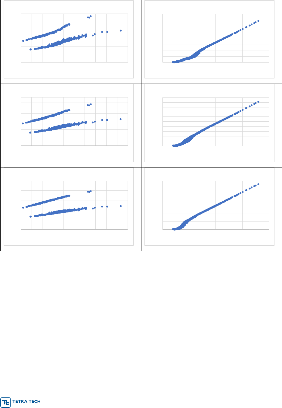
IDF Project Report September 2020
r 49
Figure 5-4. Extended Wet Detention Basin Simulation Results for Peak Outflow as a Function of Total
Storm Depth
Note: Figures on left side show closeup of responses to higher frequency, lower volume peak events; figures on right side show
responses to lower frequency extreme events.
0
0.2
0.4
0.6
0.8
1
1.2
0.5 0.6 0.7 0.8 0.9 1 1.1 1.2 1.3 1.4 1.5
Peak Flow (cfs)
Storm Depth (in)
Wet Pond Site Peak Flow at 25% imperv
0
50
100
150
200
250
300
350
400
0 5 10 15 20
Peak Flow (cfs)
Storm Depth (in)
Wet Pond Site Peak Flow at 25% imperv
0
0.2
0.4
0.6
0.8
1
1.2
1.4
1.6
1.8
0.5 0.6 0.7 0.8 0.9 1 1.1 1.2 1.3 1.4 1.5
Peak Flow (cfs)
Storm Depth (in)
Wet Pond Site Peak Flow at 50% imperv
0
50
100
150
200
250
300
350
400
450
500
0 5 10 15 20
Peak Flow (cfs)
Storm Depth (in)
Wet Pond Site Peak Flow at 50% imperv
0
0.5
1
1.5
2
2.5
0.5 0.6 0.7 0.8 0.9 1 1.1 1.2 1.3 1.4 1.5
Peak Flow (cfs)
Storm Depth (in)
Wet Pond Site Peak Flow at 80% imperv
0
100
200
300
400
500
600
0 5 10 15 20
Peak Flow (cfs)
Storm Depth (in)
Wet Pond Site Peak Flow at 80% imperv
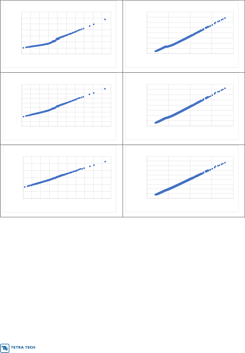
IDF Project Report September 2020
r 50
Figure 5-5. Extended Wet Detention Simulation Results for Overflow Volume as a Function of Total
Storm Depth
Note: Figures on left side show closeup of responses to higher frequency, lower volume peak events; figures on right side show
responses to lower frequency extreme events.
0
10000
20000
30000
40000
50000
60000
70000
0.5 0.6 0.7 0.8 0.9 1 1.1 1.2 1.3 1.4 1.5
Outflow Volume (cf)
Storm Depth (in)
Wet Pond Site Outflow Volume at 25% imperv
0
200000
400000
600000
800000
1000000
1200000
1400000
1600000
0 5 10 15 20
Outflow Volume (cf)
Storm Depth (in)
Wet Pond Site Outflow Volume at 25% imperv
0
10000
20000
30000
40000
50000
60000
70000
80000
90000
0.5 0.6 0.7 0.8 0.9 1 1.1 1.2 1.3 1.4 1.5
Outflow Volume (cf)
Storm Depth (in)
Wet Pond Site Outflow Volume at 50% imperv
0
200000
400000
600000
800000
1000000
1200000
1400000
1600000
0 5 10 15 20
Outflow Volume (cf)
Storm Depth (in)
Wet Pond Site Outflow Volume at 50% imperv
0
20000
40000
60000
80000
100000
120000
0.5 0.6 0.7 0.8 0.9 1 1.1 1.2 1.3 1.4 1.5
Outflow Volume (cf)
Storm Depth (in)
Wet Pond Site Outflow Volume at 80% imperv
0
200000
400000
600000
800000
1000000
1200000
1400000
1600000
1800000
0 5 10 15 20
Outflow Volume (cf)
Storm Depth (in)
Wet Pond Site Outflow Volume at 80% imperv

IDF Project Report September 2020
r 51
6.0 IMPLICATIONS FOR DESIGN
This section builds upon the previous material to provide a quantitative evaluation of the potential impacts
of changes in storm IDF relationships in three areas: channel stability, risk of road flooding, and the
general performance efficiency of urban stormwater BMPs.
6.1 CHANNEL STABILITY
The structure of a stream channel adjusts over time as it attempts to reach an approximate equilibrium
between flow energy and sediment supply. If these inputs change, then the channel will also change.
For example, in urbanizing areas where impervious surface increases, resulting in increased runoff and
greater flow energy, channels often respond by first incising and then widening, losing connection with the
floodplain, and generating large quantities of mobile sediment. These changes result in degraded habitat
and poor biology (Walsh et al., 2005).
The morphologic response of stream channels is closely related to the effective discharge or channel-
forming flow (Wolman and Miller, 1960), which integrates the sediment-carrying capacity and probability
of occurrence to evaluate the flow that, over time, transports the largest mass of sediment. Effective
discharge is closely related to bankfull discharge and is typically associated with flows that have a
recurrence frequency of once in from one to two years (Simon, 2004). One of the functions of urban
BMPs is to limit erosive flows and maintain channel stability by retaining enough water to achieve a
specified channel protection volume; in Maryland, this is based on a one-year 24-hour runoff event (MDE,
2009). Similarly, Palmer et al. (2005) state that ecologically successful stream restoration designs must
be self-sustaining systems with the ability to maintain equilibrium despite changes; thus, restoration
designs seek to ensure that the redesigned channel is consistent with expected channel-forming flows.
Current practice for both BMP and restoration design typically relies on the historic record to estimate
design flows. If future climate brings more intense precipitation and runoff at recurrence intervals
corresponding to channel-forming flows, then sediment transport capacity will increase and channel
adjustments of incision or widening can be expected as the system attempts to reach a new equilibrium.
Thus, changes in IDF relationships could threaten the resilience of stream restoration efforts, while BMPs
to control runoff might not achieve channel protection goals.
Changes in the one-year 24-hour (or 1.5-year 24-hour) flow give an indication of potential risks to stream
channel resilience but are not a direct measure of stream stability. On the other hand, a full analysis of
stability is a site-specific exercise that needs to incorporate the geometry, slope, and external sediment
supply to a stream reach in addition to the flow. As a middle way, simplified semi-quantitative tools are
useful to provide broad-scale screening of the potential effects of changes in IDF relationships on stream
stability.
The GeoTools package (Bledsoe et al., 2007; Raff et al., 2007) is designed to aid in the estimation of
erosion potential and associated risk indices. The use of these methods is demonstrated in Bledsoe and
Watson (2001) and Bledsoe (2002), among others.
The GeoTools effective discharge analysis provides two summary measures of channel stability.

IDF Project Report September 2020
r 52
• The Mobility Index (MI) is defined as
, where Q is discharge (m
3
/s), S is slope
(dimensionless), and d
50
is the median grain size (m [mm x 10-3]; Chang, 1985; Bledsoe and
Watson, 2001). MI was developed in part as a measure of channel form and stability in cases
where channel width data are unavailable.
• Specific Stream Power (ω) is defined as
, where Ω is total stream power, γ
m
is
the specific weight of the water and sediment mixture (kg), and w is the channel width (m). This
measure has also been used as an index of channel form and response (Bledsoe and Watson,
2001).
Section 4.0 developed estimates of precipitation IDF relationships under future climate in Maryland, while
Section 5.1 provided SWMM5-predicted runoff associated with future precipitation events of specified
recurrence and duration. The runoff simulations use a unit-area representation of a generic urban
landscape at varying levels of effective imperviousness. Because channel width is not explicitly specified
for each location, analysis with MI is more useful than ω for evaluating potential changes in stream
stability.
Bledsoe and Watson (2001) used MI to develop logistic regressions to predict whether a stream channel
was stable (meandering) or unstable (incising). Their model #45, which uses the base-10 logarithm of MI
and defines MI based on annual (1-year recurrence) 24-hour flow magnitude rather than bankfull flow,
classified stable meandering and incising channels with sand beds with over 95% accuracy over a
sample of 77 well-studied streams. The resulting logistic model of the probability of incision (p) is:
The logistic model results in an S-shaped curve. As MI approaches 0, p also asymptotes toward zero; as
MI approaches 1, p asymptotes towards 1. The rate of change of p relative to MI is steepest in the middle
of the range, where a small change in MI can result in a large change in p. A similar type of relationship
is expected for Maryland streams, although the regression coefficients may differ, and an equation of this
form is useful for exploring relative risk of stream instability due to climate change.
To apply the logistic model to the IDF analysis, we use for Q the peak runoff response to the 1-year
precipitation event on a 1-acre drainage area predicted by the SWMM model (bioretention setup without
presence of BMP). We use the 1-acre peak rather than daily average flow for comparative purposes
because it is the shear stress associated with the peak flow rate that determines sediment mobility during
the event; however, it is evident that the analysis of real streams with multiple contributing areas is much
more complex.
Note that Q scales with the drainage area with an approximately linear response until significant
variations in time of concentration manifest and MI thus scales approximately as the square root of the
drainage area. This indicates that as area and/or Q increases then either S must decrease or √d
50
must
increase by a proportional amount to maintain the same probability of channel stability. Results are
presented here on a 1-acre basis to explore the potential relative changes in stability under future climate.
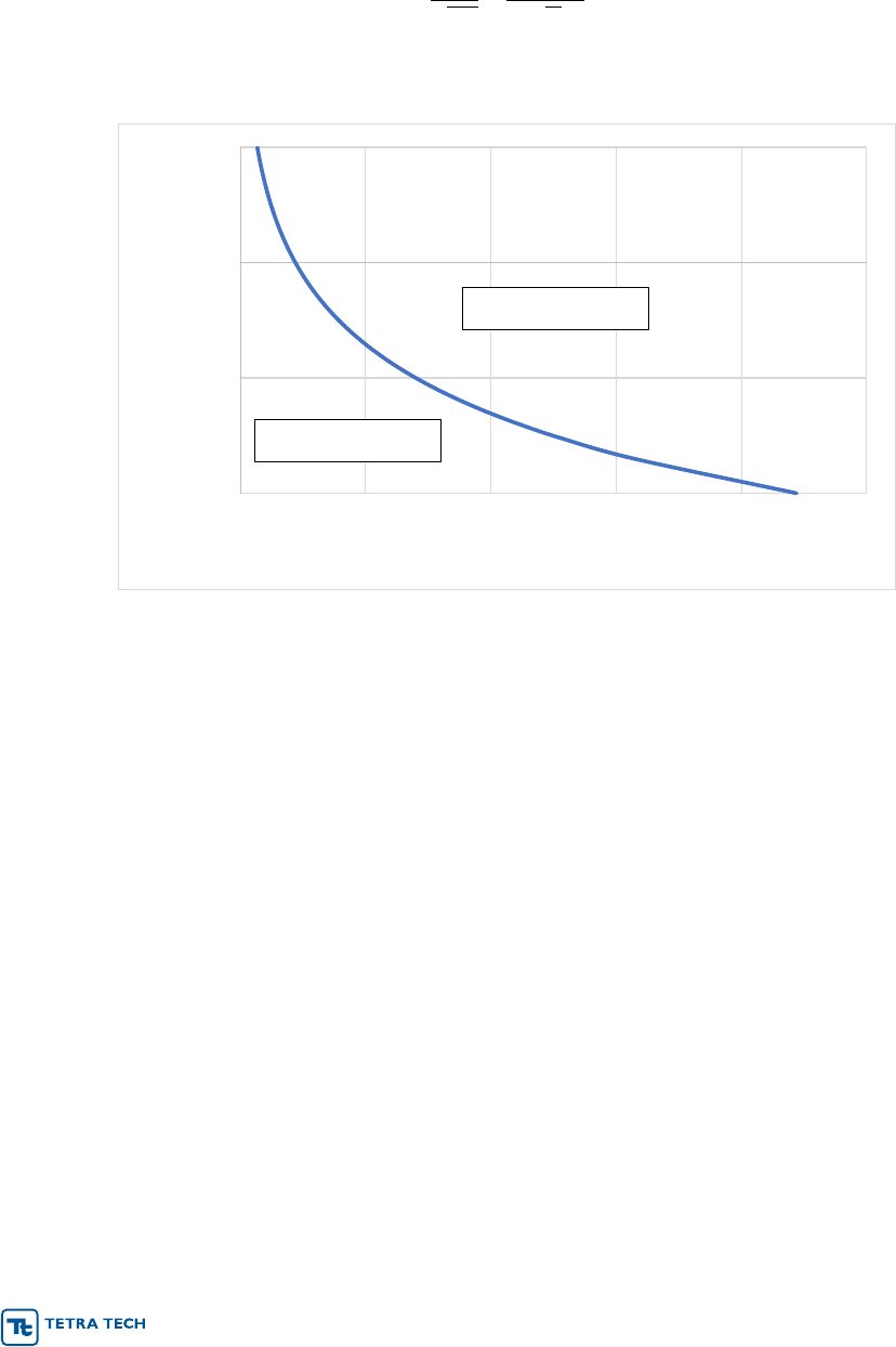
IDF Project Report September 2020
r 53
The logistic model probability representation is a function of S/√d
50
. Setting p = 0.5 defines the point of
transition from likely stable to likely incising conditions (for sand-bed streams). This occurs when
The resulting transition frontier is shown in Figure 6-1. As Q increases above the transition curve the
predicted probability of incision increases above 50%.
Figure 6-1. Stability Transition Frontier for Sand Bed Stream with 1-acre Drainage
The probability of instability increases with longer recurrence frequency and increased imperviousness,
both of which increase peak runoff. We explore results without BMPs (also applicable to stream
restoration design), with runoff control by bioretention cells, and with extended wet detention basins.
Figure 6-2, showing results without BMPs, compares predicted MI for runoff from 1 acre at 25% and 80%
imperviousness (average across all sites, with S/√d
50
= 1.75, where p = 50% corresponds to MI = 0.443.)
Each chart shows nine lines, representing historic conditions, the four selected GCMs for ca. 2055
conditions, and the four selected GCMs for ca. 2085 conditions, S/√d
50
= 1.75 is taken as an example of
a headwater stream or drainage channel at conditions near the stability limit, corresponding to, for
instance, a channel with a slope of 1.5% and a d
50
of 0.073 mm or a slope of 2.77% and a d
50
of 0.25
mm. Most future climate scenarios show an increase in MI that grows larger at longer return intervals.
0.01
0.1
1
10
0 1 2 3 4 5
Q (m
3
/s)
S/(d
50
)
0.5
Likely Unstable
Likely Stable
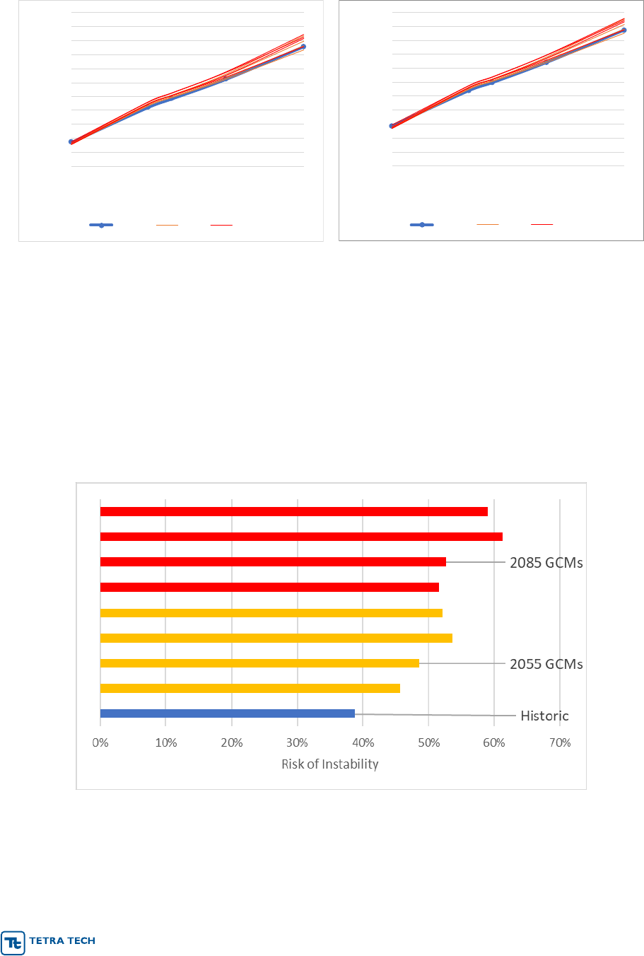
IDF Project Report September 2020
r 54
Figure 6-2. Average Mobility Index for 25% (left) and 80% (right) Impervious Cover 1-acre Parcel, S/√d
50
= 1.75 m
-0.5
For the logistic regression of Bledsoe and Watson, the 1-year 24-hr event flow results provide the
prediction of potential channel instability. Maintaining the ratio of S/√d
50
= 1.75 m
-0.5
(other ratios provide
similar, but shifted results), simulation of the probability of instability based on the 1-year recurrence peak
runoff calculated using SWMM from historic and potential future IDF curves yields the average results
across all 79 Maryland Atlas 14 stations at 25% imperviousness shown in Figure 6-3 and summarized (for
three levels of imperviousness) on the left side of Table 6-1. These probabilities increase with both
percent imperviousness and time into the future, with only historic climate conditions at 25%
imperviousness falling below the 50% target for these site conditions.
Figure 6-3. Predicted Probability of Channel Instability at 25% Imperviousness for Runoff from a 1 Acre
Site with S/√d
50
= 1.75 using the Logistic Regression of Bledsoe and Watson (2001)
0
0.1
0.2
0.3
0.4
0.5
0.6
0.7
0.8
0.9
1
1.1
0.1 1 10 100
Mobility Index
Recurrence (years)
Historic 2055 2085
0
0.1
0.2
0.3
0.4
0.5
0.6
0.7
0.8
0.9
1
1.1
0.1 1 10 100
Mobility Index
Recurrence (years)
Historic 2055 2085

IDF Project Report September 2020
r 55
Table 6-1. Probability of Channel Instability for Runoff from 1 Acre with S/√d
50
= 1.75, with and without
Bioretention BMPs
No BMP
Bioretention
Imperviousness
25%
50%
80%
25%
50%
80%
Historic
38.73%
71.59%
86.79%
34.39%
49.41%
44.78%
2055
50.01%
78.76%
90.21%
45.57%
64.51%
63.32%
2085
56.16%
82.06%
91.73%
52.04%
71.72%
71.76%
Note: Results are averages across 79 sites. Results for 2055 and 2085 are averaged across four GCMs for each site.
The right side of Table 6-1 shows the results for the same conditions but with treatment of runoff by
bioretention cells designed to current Maryland standards. Bioretention cell sizing varies with Simple
method predictions of runoff amount, which suppresses variability across percent imperviousness. For
historic climate, the probability of incision is less than 50% for all three levels of imperviousness (which
appears to corroborate the design standards); however, the probability of instability increases under
predicted future climate conditions.
Channels with lower values of S/√d
50
(e.g., with a lower slope or larger particle size) will have lower
predicted risk of instability. Results for an individual site are sensitive to the value of S/√d
50
, although the
pattern remains the same (Table 6-2). For a fine sand bed with d
50
= 0.25 mm, the S/√d
50
range
corresponds to slopes from 1.58% to 3.16%.
Table 6-2. Probability of Channel Instability for Runoff from 1 Acre Parcel with Alternative S/√d
50
at 80%
Imperviousness
No BMP
Bioretention
S/√d
50
1.0
1.5
1.75
2.0
1.0
1.5
1.75
2.0
Historic
2.96%
59.92%
86.79%
95.95%
0.37%
15.58%
44.78%
74.51%
2055
4.13%
67.75%
90.21%
97.08%
0.82%
28.53%
63.32%
86.03%
2085
4.96%
71.69%
91.73%
97.56%
1.24%
37.34%
71.76%
90.02%
Results shown above represent averages across 79 sites for which there are varying predictions of
change in the 1-year 24-hour flow. Results for individual sites are highly variable, reflecting genuine
geographic variations, statistical, and potential anomalies in the LOCA downscaling process, as well as
the effective impervious area of the drainage.
Figure 6-4 gives an illustration of the spread among individual results in the form of a histogram versus
probability bins for predicted instability (again using S/√d
50
= 1.75 as an example). All time periods have
examples that span most of the possible probability range; however, the future time periods predict a
reduction in low probability categories and an increase in high probability categories. The shift associated
with future climate is more clearly seen in a histogram that shows the percentage of cases that are
greater than a given level of probability (Figure 6-5).
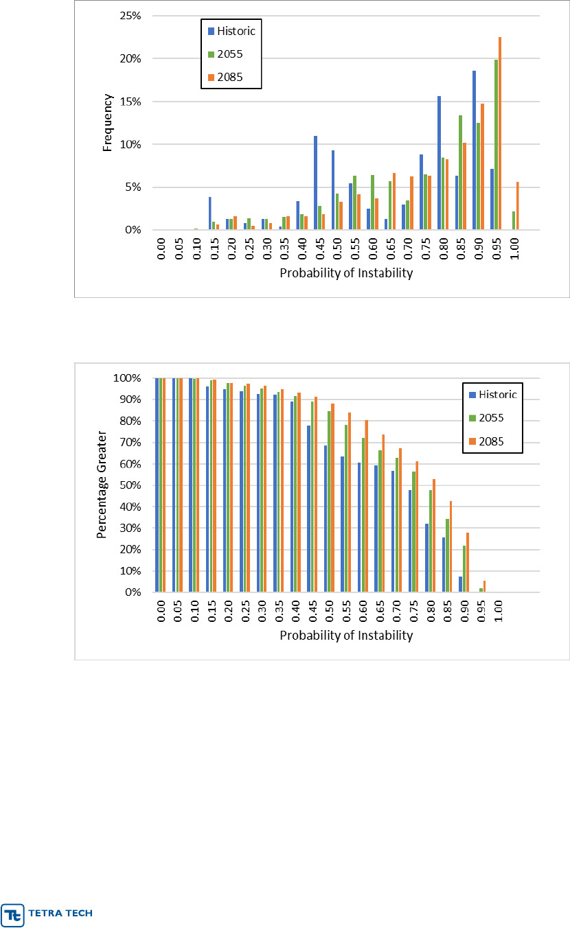
IDF Project Report September 2020
r 56
Figure 6-4. Histogram of Individual Station/GCM/Imperviousness for Probability of Channel Instability
with S/√d
50
= 1.75, 1 Acre Drainage, and no BMP
Figure 6-5. Inverse Cumulative Distribution Function (Percentage Greater than Specified Level) of
Individual Station/GCM/Imperviousness for Probability of Channel Instability with S/√d
50
= 1.75, 1 Acre
Drainage, and no BMP
An extended wet detention pond is assumed to treat a larger drainage area than a bioretention cell and
the SWMM simulations of flow through the pond use a contributing area of 25 acres, which results in
higher runoff volume. Accordingly, the value of S/√d
50
must shift to a lower value to maintain stability. To
provide comparability with the bioretention example we scale the ratio by the square root of the drainage
area. Dividing the previous example value of this ratio of 1.75 by √25 yields S/√d
50
= 0.35, which results
in an MI diagram similar to that shown above in Figure 6-2. For example, a ratio of 0.35 might
correspond to a slope of 0.55% at a d
50
of 0.25 mm.
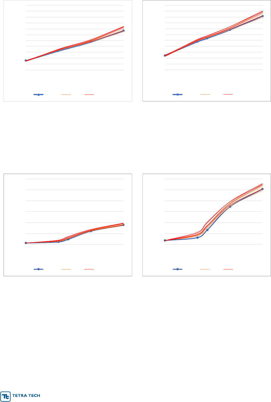
IDF Project Report September 2020
r 57
Figure 6-6. Average Mobility Index for 25% (left) and 80% (right) Impervious Cover, 25-acre Parcel,
S/√d
50
= 0.35 m
-0.5
The wet detention pond is designed to provide protection to the channel through the 10-year event, with a
margin of safety. It is thus not surprising that the MI remains low for the 1-year event at S/√d
50
=
0.35 m
-0.5
or even when S/√d
50
is increased to 1.0 due to a higher slope or decreased median particle size
(Figure 6-7). Estimated average probability of instability is summarized in Table 6-3.
Figure 6-7. Average Mobility Index for 80% Impervious Cover, 25-acre Parcel, S/√d
50
= 0.35 m
-0.5
(left)
and S/√d
50
= 1.0 m
-0.5
(right)
0
0.1
0.2
0.3
0.4
0.5
0.6
0.7
0.8
0.9
1
1.1
0.1 1 10 100
Mobility Index
Recurrence (years)
Historic 2055 2085
0
0.1
0.2
0.3
0.4
0.5
0.6
0.7
0.8
0.9
1
1.1
0.1 1 10 100
Mobility Index
Recurrence (years)
Historic 2055 2085
0
0.5
1
1.5
2
2.5
3
0.1 1 10 100
Mobility Index
Recurrence (years)
Historic 2055 2085
0
0.5
1
1.5
2
2.5
3
0.1 1 10 100
Mobility Index
Recurrence (years)
Historic 2055 2085

IDF Project Report September 2020
r 58
Table 6-3. Probability of Channel Instability for Runoff from 25-Acre Parcel based on 1-yr 24-hr Event
with Alternative Values of S/√d
50
No BMP
Wet Detention Pond
S/√d
50
0.35
1.0
0.35
1.0
25% Impervious
Historic
4.38%
99.91%
0.00%
2.53%
2055
6.76%
99.99%
0.00%
18.48%
2085
8.58%
100.00%
0.00%
37.73%
50% Impervious
Historic
31.05%
99.99%
0.00%
2.94%
2055
40.55%
99.99%
0.00%
26.53%
2085
46.16%
100.00%
0.01%
51.59%
80% Impervious
Historic
66.58%
100.00%
0.00%
2.91%
2055
74.64%
100.00%
0.00%
38.42%
2085
78.46%
100.00%
0.02%
69.33%
The analyses presented in this section indicate that relatively small increases in the magnitude of the
runoff associated with the 1-year 24-hour storm event could result in a strong increase in the risk of
channel instability. This implies that BMPs and restoration designs may not function as intended to
protect stream channels if the intensity and frequency of large storm events continues to increase.
However, the geomorphic impact on individual stream reaches will vary according to site-specific
characteristics and cannot be predicted through a generic analysis, although MI curves and estimates of
stability risk similar to those presented above could be developed for a specific site using GeoTools
(Bledsoe et al., 2007). How predictions of increased risk should be addressed also depends on other
factors, such as the useful lifespan of a design and the ability of the stream to adjust to changes as
discussed further in Section 7.0.
6.2 ROADWAY FLOODING RISK
Roadway flooding is an important public safety concern associated with changing rainfall patterns. In
many cases, road overtopping occurs when culvert capacity is exceeded. Overloaded culverts can also
result in increased exit velocities that affect stream stability. By definition, culverts are structures that
have low flexibility: once installed they are difficult and expensive to replace. It is therefore important to
include a margin of safety in culvert design, which should attempt to account for potential changes in
runoff over the design life.
The Maryland Department of Transportation, State Highway Administration (MDOT-SHA) provides
guidelines for culvert design (MDOT-SHA, 2009) and refers to the Federal Highway Administration HDS 5
(FHWA, 2012) for hydraulic calculations. MDOT-SHA (2009) establishes different levels of service
depending on road type. Culverts are designed for various storm recurrences, ranging from the 10-year

IDF Project Report September 2020
r 59
storm (peak runoff) for local streets to the 100-year storm for expressways; however, the performance of
all regulated culverts must also be examined for the 100-year flood. The Froude number, for which a
value of 1.0 would represent the point of conversion from sub-critical to critical turbulent flow at the outlet,
must not exceed 0.9 or the pre-existing Froude number, whichever is higher, as a result of the 100-year
storm. Culverts are to have a minimum diameter of 18”; 24” if the length is over 60 feet.
MDOT-SHA (2009) is not very clear on the target freeboard to be maintained between the headwater
elevation and the road surface, but references HDS 5, which calls for a freeboard of 2 feet at the design
flow. Calculation of flow through a culvert is complicated because culverts are generally a significant
constriction to watercourse cross-sectional area and are subject to a range of gradually varied and rapidly
varied flow types influenced by geometric characteristics of the culvert and those immediately upstream
and downstream. Further, culvert flow may be categorized as outflow controlled (in which the tailwater
elevation has a significant influence) or inlet control ( in which the headwater depth at the culvert has the
major influence). Culvert design calculations must simultaneously address both possibilities, leading to
complex calculations. HDS 5 recommends the use of the Federal Highway Administration program HY8
(http://www.fhwa.dot.gov/engineering/hydraulics/software/hy8/), based on Schall et al. (2012), for this
purpose.
For our analysis, we consider two designs for example. One is for a minor arterial road (which is
designed for the 50-year event) and one is for a local road (which is designed for the 10-year event). The
minor arterial representation is selected to match the Design Guideline 1 example given in FHWA (2012).
The example 50-year storm peak (from a moderate sized [125-acre] watershed) is 200 cfs; the 10-year
storm peak (from a smaller [75-acre] local watershed) is 24 cfs.
Both examples assume a 1% culvert slope and use of a concrete round culvert with a non-projecting end,
and both have an upstream invert elevation of 100 ft and road surface at a crest elevation of 110 ft. The
design must thus achieve a maximum headwater elevation of 108 ft or less after accounting for 2 feet of
freeboard. A headwater elevation just below 108 ft is obtained with a 4.5 ft diameter culvert for the minor
arterial example and a diameter of 1.5 ft for the local road. Figure 6-8 and Figure 6-9 show the full HY-8
specifications for these designs.
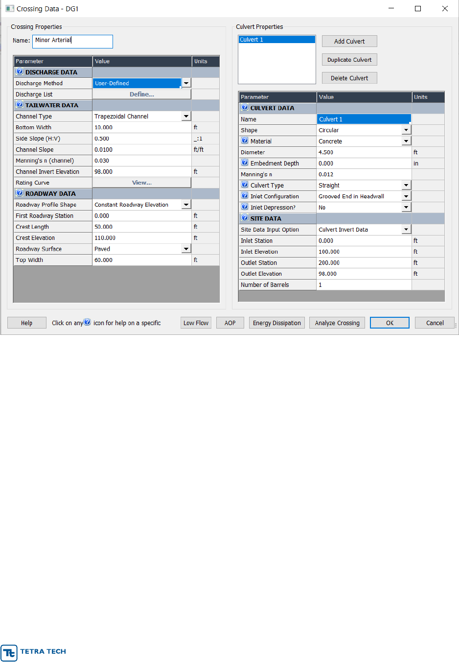
IDF Project Report September 2020
r 60
Figure 6-8. Minor Arterial Road Culvert, HY-8 Specifications
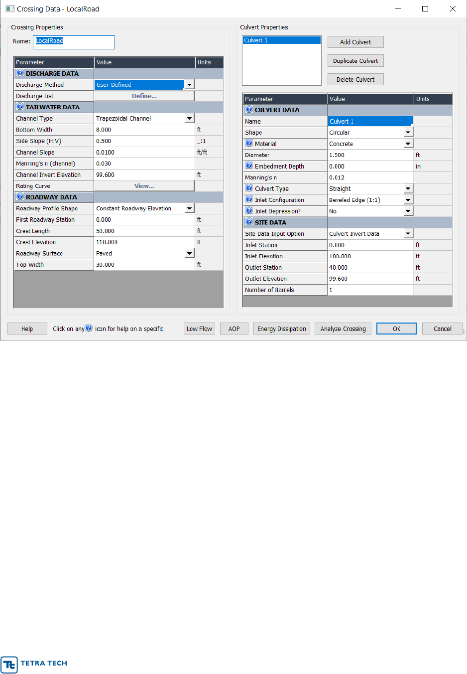
IDF Project Report September 2020
r 61
Figure 6-9. Local Road Culvert HY-8 Specifications
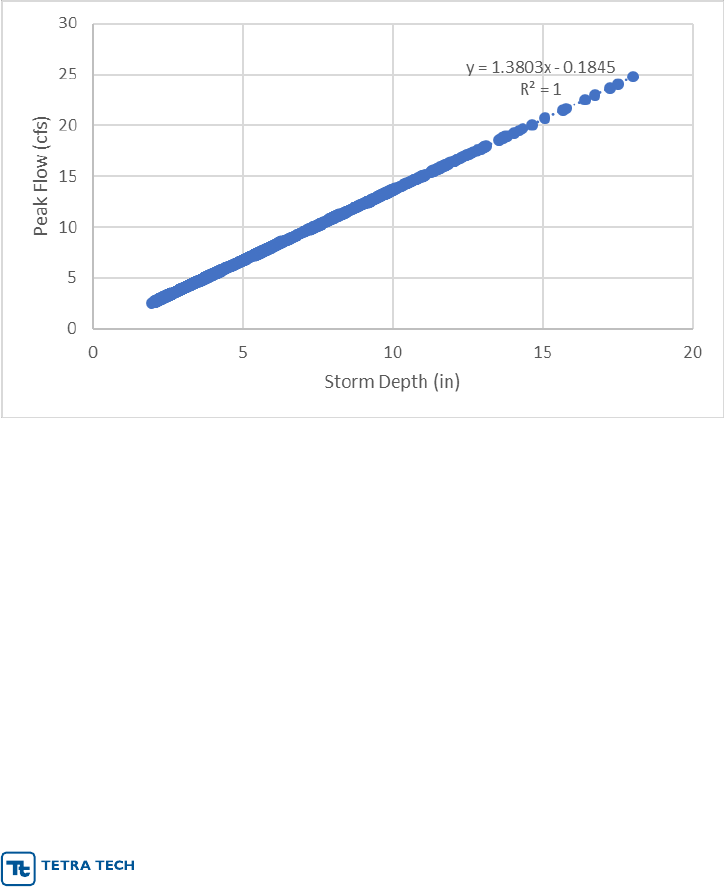
IDF Project Report September 2020
r 62
The two culverts described above meet requirements based on historic climate. We now examine
performance under potential future climate. Section 5.0 provides predictions of runoff from a unit area
urban site (at various levels of imperviousness) both with and without BMPs under present and potential
future climate regimes for 79 Maryland stations. We report here on the 80% impervious simulations –
using this extreme case for clarity of exposition. Similar relationships would be found at lower levels of
imperviousness because the imperviousness controls the peak runoff used for both current condition
design and future condition predictions.
To test culvert performance, it is necessary to convert the unit-area flows to actual flow amounts. To do
this, note that for the flows of interest (10-year recurrence and above) and high imperviousness, the
runoff flow peak is a linear function of the 24-hour rainfall event (Figure 6-10). This implies that it is
reasonable to scale the unit-area runoff results to the magnitude of the event flows used in the culvert
simulations. (Note, this ignores dissipation of the flood peak relative to variable time of concentration
across the contributing watershed, but the effect is expected to be small for a highly impervious area and
errs on the side of conservatism. We also assume that the n-year recurrence 24-hr flood event is
synonymous with the runoff from the n-year recurrence 24-hr rainfall event, ignoring potential
contributions from snowmelt.)
Figure 6-10. Relationship between Peak Flow from 1-acre (80% Impervious) and 24-hour Precipitation
Depth
We ran HY-8 at multiple flow levels ranging from 50% to 200% of the design flow (10-year for the local
road culvert and 50-year flow for the arterial culvert). Table 6-4 and Table 6-5 summarize the HY-8
results.

IDF Project Report September 2020
r 63
Table 6-4. HY-8 Results, Local Road Culvert
Total
Discharge
(cfs)
Culvert
Discharge
(cfs)
Headwater
Elevation (ft
)
Inlet Control
Depth (ft)
Outlet
Control
Depth (ft)
Tailwater
Depth (ft)
Outlet
Velocity (ft/s)
Tailwater
Velocity (ft/s)
Depth on
Road (ft)
% Design
Flow
12.0
12.0
102.64
2.64
2.31
0.50
7.31
2.92
0
50%
14.4
14.4
103.35
3.35
2.93
0.56
8.42
3.12
0
60%
16.8
16.8
104.15
4.15
3.63
0.61
9.77
3.30
0
70%
19.2
19.2
105.13
5.13
4.43
0.67
10.87
3.46
0
80%
21.6
21.6
106.30
6.30
5.32
0.72
12.22
3.61
0
90%
24.0
24.0
107.60
7.60
6.31
0.76
13.58
3.75
0
100%
26.4
26.4
109.04
9.04
7.40
0.81
14.94
3.88
0
110%
28.8
27.9
110.03
10.03
8.16
0.85
15.81
4.00
0.03
120%
31.2
28.0
110.08
10.08
8.19
0.90
15.85
4.12
0.08
130%
33.6
28.1
110.11
10.11
8.22
0.94
15.88
4.22
0.11
140%
36.0
28.1
110.14
10.14
8.24
0.98
15.90
4.33
0.14
150%
38.4
28.1
110.17
10.17
8.26
1.02
15.93
4.42
0.17
160%
40.8
28.2
110.19
10.19
8.28
1.06
15.95
4.52
0.19
170%
43.2
28.2
110.22
10.22
8.30
1.10
15.97
4.61
0.22
180%
45.6
28.3
110.24
10.24
8.31
1.13
15.98
4.69
0.24
190%
48.0
28.3
110.26
10.26
8.33
1.17
16.00
4.78
0.26
200%

IDF Project Report September 2020
r 64
Table 6-5. HY-8 Results, Minor Arterial Culvert
Total
Discharge
(cfs)
Culvert
Discharge
(cfs)
Headwater
Elevation (ft)
Inlet Control
Depth (ft)
Outlet
Control
Depth (ft)
Tailwater
Depth (ft)
Outlet
Velocity (ft/s)
Tailwater
Velocity (ft/s)
Depth on
Road (ft)
% Design
Flow
100
100.00
104.29
4.29
2.11
1.60
12.66
5.81
0
50%
120
120.00
104.86
4.86
2.92
1.79
13.20
6.17
0
60%
140
140.00
105.49
5.49
4.29
1.97
13.69
6.49
0
70%
160
160.00
106.20
6.21
5.11
2.13
14.14
6.77
0
80%
180
180.00
107.01
7.01
6.00
2.30
14.54
7.03
0
90%
200
200.00
107.90
7.90
6.97
2.45
14.89
7.27
0
100%
220
220.00
108.88
8.88
8.01
2.60
15.10
7.49
0
110%
240
240.00
109.94
9.94
9.11
2.75
15.45
7.69
0
120%
260
244.98
110.22
10.22
9.43
2.88
15.73
7.88
0.22
130%
280
247.53
110.36
10.36
9.58
3.02
15.88
8.06
0.36
140%
300
249.67
110.48
10.48
9.71
3.15
16.00
8.23
0.48
150%
320
251.57
110.59
10.59
9.83
3.28
16.11
8.38
0.59
160%
340
253.33
110.69
10.69
9.94
3.40
16.21
8.54
0.69
170%
360
254.97
110.78
10.78
10.04
3.53
16.31
8.68
0.78
180%
380
256.52
110.87
10.87
10.14
3.65
16.40
8.82
0.87
190%
400
257.99
110.96
10.96
10.23
3.76
16.48
8.95
0.96
200%
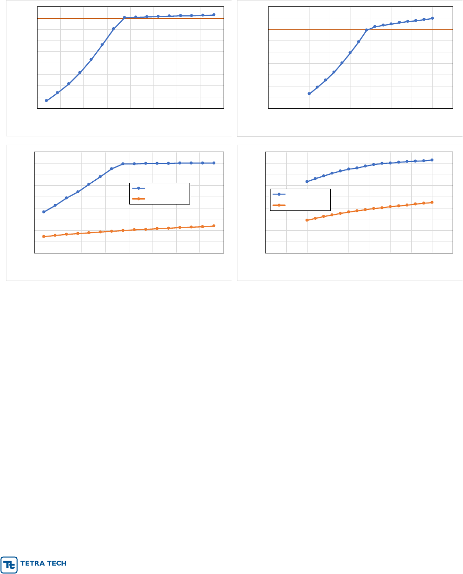
IDF Project Report September 2020
r 65
HY-8 predictions of headwater depth and outlet velocity as a function of discharge are exactly fit by two
second-order polynomials of the form Y = β
2
X
2
+ β
1
X + β
0
, with a break at the elevation where the road
is overtopped (Figure 6-11 and Table 6-6). This allows prediction for any discharge within the polynomial
fitting range (i.e., from 50% to 200% of the design flow).
The bottom portion of Figure 6-11 shows how the outlet and tailwater velocities, which may impact
downstream channel stability, increase with flow.
Figure 6-11. Relationship of Headwater Elevation and Outlet Velocity to Flow for Local Road (Left) and
Minor Arterial (Right) Culvert Designs
102
103
104
105
106
107
108
109
110
111
10 15 20 25 30 35 40 45 50
Headwater (ft)
Flow (cfs)
103
104
105
106
107
108
109
110
111
112
0 50 100 150 200 250 300 350 400 450
Headwater (ft)
Flow (cfs)
0
2
4
6
8
10
12
14
16
18
10 15 20 25 30 35 40 45 50
Velocity (ft/s)
Flow (cfs)
Outlet Velocity
Tailwater Velocity
0
2
4
6
8
10
12
14
16
18
0 50 100 150 200 250 300 350 400 450
Velocity (ft/s)
Flow (cfs)
Outlet Velocity
Tailwater Velocity
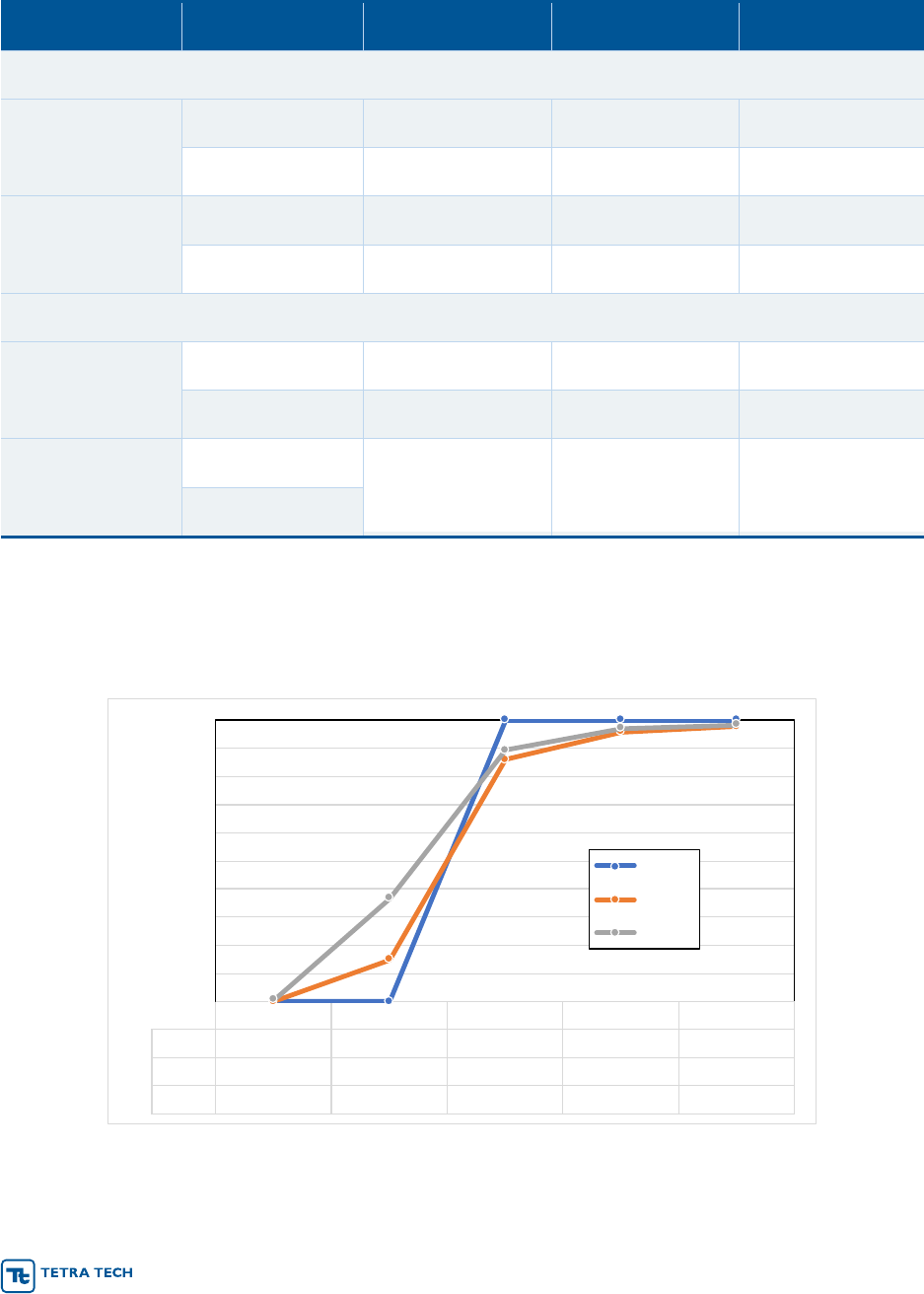
IDF Project Report September 2020
r 66
Table 6-6. Polynomial Coefficients for Relationship of Headwater Elevation and Outlet Velocity to Flow
Design
Range
β
2
(X
2
)
β
1
(X)
β
0
Headwater Elevation
Local Road
Below Road
1.3496E-02
-0.0741
101.5943
Above Road
-2.4238E-04
0.0302
109.3666
Minor Arterial
Below Road
1.0610E-04
0.0042
102.8152
Above Road
-1.0268E-05
0.0120
107.8073
Outlet Velocity
Local Road
Below Road
3.7781E-03
0.3856
2.1323
Above Road
-2.1833E-04
0.0265
15.2324
Minor Arterial
Below Road
-4.4243E-05
0.0343
9.7418
Above Road
The polynomial relationships in Table 6-6 allow prediction of response to future runoff events of different
recurrence frequencies (Figure 6-12 and Figure 6-13). Results are averages for all 79 Atlas 14 stations.
The historic simulations are based directly on Atlas 14 IDF results, while the future climate percentages
summarize results from four different downscaled GCMs per station and time.
Figure 6-12. Predicted Frequency of Road Overtopping under Future Climate, Local Road Culvert
Note: Design of local road culvert is based on the 10-year event.
5-yr 10-yr 25-yr 50-yr 100-yr
Historic
0.00% 0.00% 100.00% 100.00% 100.00%
2055
0.00% 14.87% 86.08% 95.89% 97.78%
2085
0.63% 36.71% 89.24% 97.15% 98.42%
0%
10%
20%
30%
40%
50%
60%
70%
80%
90%
100%
Percent Overtopping Road
Historic
2055
2085

IDF Project Report September 2020
r 67
Figure 6-13. Predicted Frequency of Road Overtopping under Future Climate, Minor Arterial Culvert
Note: Design of the minor arterial culvert is based on the 50-year event,
As expected, the culverts do not result in road overtopping at their design storm recurrence under historic
climate (10-year recurrence for the local road culvert and 50-year recurrence for the minor arterial
culvert.) The local road culvert results in road flooding at all stations for the 25-year event under historic
climate, whereas the minor arterial culvert exceeds the target freeboard elevation (2 feet below the road
surface) for the 100-year event but does not cause road flooding until flows are greater than the 100-year
event.
The predicted future climate results never reach 100% overtopping because they are based on a
statistical analysis of multiple GCMs that includes some instances where future extreme flows are not
predicted to increase. The key result is the predicted future response to the design event for each
culvert. For the local road culvert designed for the 10-year event, the risk of road overtopping during such
an event is nearly 15% by 2055 and 37% by 2085. For the minor arterial culvert designed for the 50-year
event, the risk of overtopping during such an event is 16% by 2055 and 30% by 2085.
Per MDOT-SHA (2009), all culverts have a minimum service life of 50 years and a service life of at least
75 years if the roadbed width is greater than 27 feet, so the results suggest that design criteria may need
to be adjusted to account for future climate. Results for individual sites will of course vary according to
the local climate and the characteristics of specific culverts and roads.
6.3 URBAN BMP PERFORMANCE
Water quality BMPs are used to mitigate existing or prospective impacts of land-use change and other
human activities on water quality. BMPs are typically implemented through regulations and design
guidance based on observations and assessment of existing problems (e.g., flooding, or bacterial
impairment in a monitored waterbody) or on anticipation of potential problems based on experience with
similar sites (e.g., expected impacts from new urban development). These decisions generally assume
that BMPs will function as observed under historical climate, weather, and hydrological conditions. For
instance, design requirements for water quality BMPs are typically based on achieving a level of control
10-yr 25-yr 50-yr 100-yr 200-yr 500-yr
Historic
0.00% 0.00% 0.00% 0.00% 100.00% 100.00%
2055
0.00% 1.27% 16.14% 50.00% 76.27% 89.56%
2085
0.00% 4.43% 29.75% 62.34% 81.01% 88.29%
0%
10%
20%
30%
40%
50%
60%
70%
80%
90%
100%
Percent Overtopping Road
Historic
2055
2085

IDF Project Report September 2020
r 68
for a design rainfall event with a given probability of occurrence, based on the past record of observed
rainfall. This approach assumes that the underlying statistical properties of historical climate (e.g.,
average and variability) will remain unchanged in the future. From a statistical perspective, this is known
as a stationary system. If the underlying conditions change, then the assumptions built into design
criteria may be inappropriate, and the performance of BMPs may be less protective of waterbodies than
intended.
Implicit assumptions about climate are built into guidance and regulations for both systems of BMPs and
the design of individual BMP types. We consider first how future climate may affect systems of BMPs and
then discuss design guidance for individual BMPs. Ultimately, it is the net effect of systems of BMPs that
control impacts on water quality.
Maryland Department of the Environment’s (MDE) 2000 Stormwater Design Manual presented
calculations for a Water Quality volume (WQv) and a channel protection volume (CPv) for the design of
stormwater BMPs. With the 2009 revisions to the Design Manual, MDE moved to the more holistic
approach of Environmental Site Design (ESD), which combines the WQv and CPv objectives to produce
a unified approach to stormwater design and management based on the net effects of all stormwater
controls present on a site (MDE, 2009, Chapter 5).
6.3.1 BMP Systems: Environmental Site Design
The general concept of ESD is to control runoff from a developed site in response to the 1-year 24-hour
storm so that it is no greater than the runoff that would be expected for the same site with a cover of
undeveloped woods in good condition, considering the distribution of hydrologic soil groups on the site.
ESD does not require detailed simulation modeling of developed and undeveloped conditions. Rather, it
provides a simplified approach based on the relative change in Curve Number used in the National
Resources Conservation Service TR-55 method (NRCS, 1986). The difference in responses to the 1-yr
24-hr event determines the excess runoff that needs to be treated (Q
E
). In units of depth, Q
E
= P
E
x R
V
.
R
V
is the surface runoff fraction, defined as R
V
= 0.005 + 0.009 x I, where I is the impervious fraction
expressed as a percentage. P
E
is then the excess rainfall amount that needs to be treated. Rather than
calculating P
E
simple lookup tables are provided (one for each of the four hydrologic soil groups, A, B, C,
and D). P
E
is listed in the table in increments of 0.2 inches and imperviousness in increments of 5% and
incorporates a single assumption about the 1-yr 24-hr storm across all of Maryland, so the answer is not
exact, but is sufficient to achieve the desired level of control on average, especially when weighted across
multiple subareas of a site with differing soil and development characteristics.
The approach of controlling site runoff to levels expected for woods in good condition is in theory climate
neutral because both developed and woods runoff will change if climate changes. However, the table
that is used to determine P
E
is rooted in specific assumptions about the magnitude of the 1-yr 24-hr storm
event that may not hold under future climate conditions.
We investigated how climate change might affect design criteria by examining the changes in
precipitation and the resulting difference in runoff between developed and good condition woods, as
predicted by TR-55, under future climate scenarios for the 79 NOAA Atlas 14 stations for which we have
developed estimates of the future 1-yr 24-hr event.
The TR-55 method (NRCS, 1986) predicts runoff (Q, inches) via the curve number equation as

IDF Project Report September 2020
r 69
where P is the 24-hr precipitation depth (inches) and S = 1000/CN – 10, where CN is the Curve Number.
CN assumptions for ESD are shown in Table 2-1. CNs for developed land were calculated as a weighted
mixture of the CN for connected impervious area (98) and that for open space in good condition.
Table 6-7. Curve Numbers for Environmental Site Design Simulations
Land Use
Hydrologic Soil Group
A
B
C
D
Woods, good
condition
38
55
70
77
Developed, 25%
Impervious
54
70
80
85
Developed, 50%
Impervious
69
80
86
89
Developed, 80%
Impervious
86
91
93
94
The runoff predicted by the CN method as well as the difference between runoff for developed land and
good condition woods for a given hydrologic soil group and impervious percentage is an exact second-
order polynomial function of P, as shown in Figure 2-4. This allows direct calculation of the implications
of both spatial variability and magnitude of change in the 1-yr 24-hr event.
Figure 6-14. Curve Number Prediction of Runoff as a Function of Precipitation for Hydrologic Group D
Soils, Developed Land at 80% Imperviousness
Note: Polynomial equation represents the difference between runoff from developed land and runoff from woods in
good condition.
y = -0.0424x
2
+ 0.5531x - 0.0085
0
1
2
3
4
5
6
0 1 2 3 4 5 6 7
Runoff (in)
Precipitation (in)
Woods
Developed
Difference

IDF Project Report September 2020
r 70
The 1-yr 24-hr event is predicted to increase, on average, over the course of the 21
st
century. The
magnitude of the difference between runoff from developed land and woods in good condition (the
theoretical Q
E
) will also tend to increase, as shown for example in Table 6-8. (The statistics are based on
79 stations and four climate scenarios for each future time.) This suggests a possible need to adjust ESD
P
E
table in MDE (2009) in the future; however, the predicted changes in Q
E
are small.
Table 6-8. Treatment Volume (Q
E
, inches) for Historic and Predicted Future Climate for Hydrologic Group
D Soils, Developed Land at 80% Imperviousness
Time
Minimum
Maximum
Average
Median
Historic
0.94
1.24
1.13
1.16
2055
0.91
1.42
1.19
1.21
2085
0.94
1.43
1.22
1.24
Of more relevance than how the theoretical Q
E
may change over time with runoff from both undisturbed
woods and developed sites calculated under a non-stationary climate is how the predicted future excess
runoff compares to the Q
E
that would be calculated using the tables in MDE (2009). This provides an
indication of the extent to which existing ESD regulations may be sufficient to achieve the desired level of
protection in the future. These results are provided in Table 6-9 through Table 6-12. In these tables a
positive result means that the calculated treatment volume (the difference between runoff from developed
land and good condition woods) is greater than the Q
E
as calculated from the methods in Chapter 5 of
MDE (2009) leading to a shortfall in treatment, while a negative result means that Q
E
provides a margin
relative to the site-specific target. The “Percent Exceeding” column is the percentage of trials
(combinations of GCMs and stations) where the site-specific need for volume control is greater than Q
E
.
Table 6-9. Relationship of Excess Stormwater Volume to Q
E
Calculated using Environmental Site Design
Procedure from 2009 Design Manual (MDE, 2009) – Hydrologic Soil Group A
Time
Minimum
Maximum
Average
Median
Percent
Exceeding
80% Impervious, Q
E
=1.85
Historic
-0.94
-0.25
-0.51
-0.45
0.00%
2055
-1.00
0.28
-0.36
-0.33
4.50%
2085
-0.93
0.31
-0.28
-0.24
14.00%
50% Impervious, Q
E
=0.90
Historic
-0.63
-0.25
-0.40
-0.37
0.00%
2055
-0.66
0.07
-0.31
-0.30
1.10%
2085
-0.62
0.08
-0.27
-0.25
1.80%
25% Impervious, Q
E
= 0.44
Historic
-0.40
-0.26
-0.32
-0.31
0.00%
2055
-0.41
-0.12
-0.29
-0.28
0.00%
2085
-0.40
-0.12
-0.27
-0.26
0.00%

IDF Project Report September 2020
r 71
Table 6-10. Relationship of Excess Stormwater Volume to Q
E
Calculated using Environmental Site
Design Procedure from 2009 Design Manual (MDE, 2009) – Hydrologic Soil Group B
Time
Minimum
Maximum
Average
Median
Percent
Exceeding
80% Impervious, Q
E
=1.69
Historic
-0.53
0.10
-0.13
-0.07
19.50%
2055
-0.59
0.53
0.00
0.03
59.10%
2085
-0.52
0.55
0.07
0.11
67.50%
50% Impervious, Q
E
=0.90
Historic
-0.33
0.10
-0.05
-0.02
28.00%
2055
-0.37
0.41
0.03
0.06
66.80%
2085
-0.32
0.42
0.08
0.11
74.10%
25% Impervious, Q
E
= 0.44
Historic
-0.19
0.05
-0.04
-0.02
22.90%
2055
-0.22
0.23
0.01
0.02
63.60%
2085
-0.19
0.24
0.04
0.06
72.20%
Table 6-11. Relationship of Excess Stormwater Volume to Q
E
Calculated using Environmental Site
Design Procedure from 2009 Design Manual (MDE, 2009) – Hydrologic Soil Group C
Time
Minimum
Maximum
Average
Median
Percent
Exceeding
80% Impervious, Q
E
=1.54
Historic
-0.47
-0.06
-0.20
-0.17
0.00%
2055
-0.51
0.21
-0.12
-0.10
13.20%
2085
-0.47
0.22
-0.08
-0.05
30.50%
50% Impervious, Q
E
=0.90
Historic
-0.29
0.01
-0.10
-0.07
3.10%
2055
-0.32
0.21
-0.04
-0.02
35.50%
2085
-0.29
0.21
-0.01
0.01
55.00%
25% Impervious, Q
E
= 0.33
Historic
0.00
0.18
0.12
0.13
98.40%
2055
-0.02
0.31
0.15
0.16
99.50%
2085
0.00
0.31
0.17
0.19
99.60%

IDF Project Report September 2020
r 72
Table 6-12. Relationship of Excess Stormwater Volume to Q
E
Calculated using Environmental Site
Design Procedure from 2009 Design Manual (MDE, 2009) – Hydrologic Soil Group D
Time
Minimum
Maximum
Average
Median
Percent
Exceeding
80% Impervious, Q
E
=1.39
Historic
-0.45
-0.15
-0.26
-0.23
0.00%
2055
-0.48
0.04
-0.20
-0.18
1.20%
2085
-0.45
0.05
-0.16
-0.14
1.80%
50% Impervious, Q
E
=0.90
Historic
-0.32
-0.10
-0.18
-0.16
0.00%
2055
-0.35
0.04
-0.14
-0.13
1.60%
2085
-0.32
0.05
-0.11
-0.10
4.70%
25% Impervious, Q
E
= 0.33
Historic
0.02
0.17
0.11
0.13
100.00%
2055
0.00
0.26
0.14
0.15
100.00%
2085
0.02
0.27
0.16
0.17
100.00%
The calculations reveal a few anomalies. For historic conditions for D soils and 25% impervious the
calculated difference between runoff from developed land and good conditions woods is always greater
than Q
E
, and this is also almost always the case for C soils at 25% impervious, although the magnitude of
the difference is small. This is primarily due to the coarse resolution of the simplified statewide tables in
Chapter 5 of MDE (2009) that yields approximate P
E
values only in 0.2-inch increments. For example,
this results in P
E
and Q
E
being identical for A, B, C, and D soils at 50% impervious.
The percent of cases in which Q
E
calculated under current design guidance does not provide sufficient
control volume to match forest conditions does tend to increase for future climate, but, except for B soils,
the change in percentage is generally small. Perhaps the most important result is that the magnitude of
the difference between the calculated treatment need and Q
E
is small, even under 2085 conditions. The
largest average difference (2085 for C soils at 25% impervious) is 0.17 inches. Further, the biggest
estimates of untreated runoff depth are associated with instances in which the statewide method already
tends to underestimate the need. Where the 2085 average is greater than zero, the largest increase
relative to the larger of the calculated need and Q
E
is only 0.08 inches.
6.3.2 Design of Individual Practices
While the focus of urban stormwater management in Maryland has changed to ESD, MDE (2009) also
provides design guidance for individual BMPs based on WQv and CPv – although the net effect of all
practices on a site must still meet ESD objectives. Meeting ESD objectives will typically occur through a
mix of BMPs of different types, each of which will have its own hydrologic and pollutant removal
characteristics.

IDF Project Report September 2020
r 73
Unlike ESD, the design guidance for individual practices such as bioretention continues to recognize a
separate WQv. The WQv is defined as the storage needed to capture and treat runoff from the 90
th
percentile (24-hr) rainfall event. MDE (2009) defines this event as equivalent to 1 inch in the eastern part
of Maryland and 0.9 inches in the western four counties. Thus, the guidelines for BMP design are also
tied to specific assumptions about historic climate, which may or may not be appropriate in the future.
Storm event runoff in excess of the WQv can bypass treatment altogether (as in BMPs based on
infiltration) or be subject to reduced treatment efficiency due to less contact time (as in BMPs based on
filtration or retention). Incomplete water quality treatment of runoff in excess of the WQv is expected;
however, if the fraction of annual runoff that exceeds the WQv increases then the total pollutant removal
efficiency will be less than expected.
As noted above in Section 4.0, we found no consistent prediction of an increase in the magnitude of the
90
th
percentile event across Maryland. In many cases, the future 90
th
percentile event was predicted to
be less than the historic event. Simulations of the response of bioretention (designed for the historic
WQv) to future 90
th
percentile events and found that the median change across all sites and scenarios
resulted in a decline of 18% in total outflow by 2055 and 12% by 2085 (Section 5.2). (All these results are
conditional on the LOCA statistical downscaling process and may differ using other approaches.)
The projected future results suggest that the bioretention BMP is likely to maintain (or even improve)
pollutant removal efficiency in future for the majority of individual storm events. However, most climate
simulations indicate that annual average total precipitation volume will increase in future, even where
there is no consistent increase in the 90
th
percentile event. That indicates a situation where a greater
fraction of annual precipitation is packed into the more extreme events above the 90
th
percentile. Runoff
simulations suggest that the magnitude of these lower frequency events will increase over time and that
the change will be greater for more extreme events. This will result in an increase in treatment bypass
under such events, which could decrease the long-term average water quality performance of BMPs.
The extended wet detention results in Section 5.3 also show that, on average, the volume of the 90
th
percentile WQv event is predicted to decline under future climate, which would result in longer detention
time and potentially greater pollutant removal. However, for larger events with recurrence intervals of one
year or greater the predicted total flow through and the peak outflow from extended wet detention ponds
tends to increase, resulting in reduced treatment times. The predicted changes in the performance of wet
detention ponds and bioretention are thus similar. Bioretention does have an advantage of more flexibility
if climate forecasts turn out to be incorrect as it is generally easier and less expensive to expand
bioretention than to rebuild detention basins.

IDF Project Report September 2020
r 74
(This page left intentionally blank.)

IDF Project Report September 2020
r 75
7.0 DISCUSSION
7.1 POTENTIAL USE OF CONTINUOUS SIMULATION
A comprehensive analysis of the implications of future changes in the cumulative distribution function of
rainfall events on BMP performance may require the use of continuous simulation, not just analysis of the
response to events of a specified occurrence. Continuous simulation is outside the scope of the current
work, which is focused on the IDF analysis. A detailed analysis should also represent the full details of
realistic site layouts.
An example of such a study (in which the author of this report was a participant) is provided by Job et al.
(2018). Job et al. used continuous model simulations to evaluate site conditions and BMP performance
under future climate conditions in five U.S. locations, including Harford County, MD. The analysis
provides insights into the potential impacts of changes in the characteristics of precipitation time series
(rather than just extreme events) on stormwater infrastructure performance and allows comparison of how
the responses may differ between conventional stormwater detention and GI practices.
Job et al. used the Hydrologic Simulation Program – FORTRAN (HSPF) model (Bicknell et al., 2004) to
simulate hourly unit-area time series of runoff and pollutant loads (total suspended solids, total nitrogen,
and total phosphorous) from pervious and impervious land. Future climate scenarios were developed
from the current time series using dynamically downscaled GCMs. Realistic site layouts and associated
stormwater management infrastructure were simulated using the System for Urban Stormwater Treatment
and Analysis Integration (SUSTAIN) model (Shoemaker et al., 2009), a decision support system and
modeling tool. Hourly output is provided by SUSTAIN for each individual BMP and at the site outlet.
The SUSTAIN stormwater management scenarios considered five types of developed land use:
residential, commercial, mixed-use, ultra-urban, and green street areas combined with a variety of
stormwater BMPs, ranging from gray storage infrastructure to GI designs consistent with local design
standards, requirements, and guidance.
Each stormwater management approach was modeled under current and various projected future climate
scenarios for the mid-21st century and evaluated for pollutant removal and ability to match pre-
development hydrology. The site’s practices were then modified to achieve the same or better
performance as under current climate using SUSTAIN’s optimization function to identify the lowest cost
alternative. For the Harford County, MD study area, Job et al. modified the initial designs using two
different management strategies – increasing the size of the structural storage practices and addressing
water quality performance gaps by incorporating additional distributed GI practices into the site.
Gray and green BMP systems generally removed more total runoff volume and pollutant mass under
future increases in precipitation and runoff compared to current conditions. However, overall site export
rates of runoff volume and pollutant mass still increased (i.e., BMPs did not remove 100% of the
additional runoff/pollutant load resulting from increased precipitation) despite better volume/mass
removal. Changes in large storm event runoff show that BMPs designed for current conditions will likely
not mitigate increases in stormwater runoff and associated downstream channel erosion and flooding
impacts under projected future conditions. Thus, there may be a need for adapting site stormwater
infrastructure to future precipitation conditions to protect downstream water resources. Sites may also
need to be configured to be adaptable in the first place to allow for the placement of additional stormwater
treatment if needed in the future.

IDF Project Report September 2020
r 76
Job et al. found that increasing BMP size/volume can mitigate the potential increases in flow, runoff
volume, and pollutant loads, but larger BMPs result in increased costs. The most difficult performance
measure to mitigate was usually control of large flooding event outflows, suggesting that site designs will
need greater temporary volume storage and/or reconfiguration of outlet structures to mitigate flooding and
channel erosion risk in locations where the magnitude of extreme events is expected to increase.
Overall, approaches to stormwater management that combined both conventional and GI elements
tended to have the best combined cost resiliency. GI also provides an advantage in flexibility, because it
typically has a shorter design life before rehabilitation is required – so it would be possible to commit less
investment now and use an adaptive, incremental approach as the climate evolves. There is an ongoing
need for additional detailed, site-specific continuous simulation studies to fully understand the ways in
which BMPs, stormwater conveyance infrastructure, and receiving streams may respond to potential
future climate conditions.
7.2 ADAPTATION OF BMPS IN A CHANGING CLIMATE
Stormwater management attempts to ensure desirable outcomes in the face of uncertain conditions. The
presence of uncertainty is typically addressed through a risk analysis approach in which an attempt is
made to minimize the probability of adverse outcomes. Traditional engineering risk assessment is based
on a summary of the environmental conditions the project is likely to face (based on an implicit
assumption that the past is an adequate guide to the future) accompanied by the addition of a margin of
safety to protect against failure.
Climate change introduces a new level of complexity. Despite significant advances in climate science
and modeling, and clearer understanding of many key aspects of climate, it is not currently possible to
forecast long-term, local-scale changes in climate with accuracy. Key challenges include differing levels
of confidence in projections of future climate changes at spatial and temporal scales relevant to resource
managers, variability in projecting the effects of climate change and management activities on the
environment, and potential nonlinear or abrupt changes (Dessai and Hulme, 2004; West et al., 2012).
These uncertainties must be acknowledged, together with the recognition that climate change impacts will
present an evolving, moving target throughout the coming century. It is common for managers to cite the
high uncertainties associated with climate change projections as an obstacle to making adaptation
decisions (Weaver et al. 2013; Hoffman et al. 2014). A key realization is that, while decision-making
under large climate change uncertainties can be difficult, uncertainty is not equivalent to knowing nothing
(Hoffman et al. 2014). There is a lot we know, and a large body of research and case studies that can be
drawn upon to inform adaptation planning.
At the watershed/neighborhood scale, water quality protection plans typically involve a mix of gray and
green practices specified to achieve a desired level of performance, with varying degrees of resilience
and adaptability to change. It is important to evaluate the resilience of individual practices; however, what
really matters is the resilience of the overall water quality protection plan. A typical plan will combine
BMPs with varying degrees of resilience. BMPs that have low resilience and/or adaptability may well
have a significant role in a water quality protection plan, but should be incorporated primarily to address
short-term issues that must be addressed now and for which changing circumstances in the future are not
a major concern (for example, containing and controlling runoff from a contaminated industrial site).
Uncertainty in future IDF relationships introduces uncertainty into assessment of risk and vulnerability
associated with engineering designs. One approach used to minimize potential future risk is conservative

IDF Project Report September 2020
r 77
design criteria. For instance, New York City’s climate resiliency guidelines suggest that the current 50-
year IDF curve should be used as a proxy for the future 5-year storm for the 2080s and on-site
detention/retention systems should be designed to retain the volume associated with the current 50-year
curve (NYC MORR 2019). The Federal Highway Administration (FHWA) has proposed a tiered
framework with five levels of analysis depending on the analysis of the risks of a project and its hydrologic
service life (Kilgore et al. 2016). Where risk is high (based on asset criticality, vulnerability, and cost) and
anticipated service life is long, an analysis of potential hydrologic responses to changes in both land use
and climate with associated confidence intervals is needed (e.g., 68% confidence interval for service life
between 30 and 75 years). Multiple types of model and data uncertainty contribute to uncertainty in
estimating runoff; however, a key source of uncertainty for prospective analysis is the difference between
different climate models and greenhouse gas emission scenarios. FHWA recommends evaluation over
multiple climate models/scenarios to address this source of uncertainty, focusing on the potential change
in the NOAA Atlas 14 analysis of 24-hour duration precipitation amounts (and associated confidence
intervals) for appropriate recurrence intervals.
In general, climate-smart strategies must address both how change will affect stressors of concern and
how change may alter the functionality of management actions (e.g., West et al., 2018). A key
component of climate-smart strategies is implementing BMPs that will function as intended under future
conditions. In practice, assessing resilience involves selecting an appropriate range of potential climate
futures (hazards) and assessing the associated vulnerabilities and risks of the BMPs incorporated in a
plan. While many lines of evidence can be assembled as to the likely response of BMPs to climate
change, future climate conditions are subject to uncertainty. Further, the performance of BMPs may
change in unexpected ways. It is therefore important to both select BMP strategies that appear to be
robust under the range of likely future climate conditions and to monitor their effectiveness over time.
Flexibility and adaptive management are hallmarks of sound adaptation planning and decision making
under high degrees of uncertainty regarding future conditions. Three general principles applicable to
BMPs and climate change are:
• Remain as flexible as possible—Managing under uncertainty can be a major impediment to
implementing adaptation, making the flexibility of candidate strategies a recommended criterion
for selection (Hoffman et al. 2014). For BMPs, flexibility and adaptability are key considerations.
• Look for no-regrets opportunities—Low-regret or no-regret strategies and options are widely
recommended. They benefit resource management regardless of whether and how climate
changes or provide a wide array of benefits (Wilby et al. 2010; Hallegatte 2009; Hoffman et al.
2014). A related principle is to consider safety-margin strategies that build in additional capacity
to accommodate future climate changes because the cost of doing so now is relatively small
(mainly a design change), while the cost of increasing capacity after implementation can be high.
• Look for robust solutions—Adaptation strategies should be implemented in a way that explicitly
acknowledges future uncertainties and hedges the success of the adaptations against a wide
range of plausible but uncertain future climatic conditions. Options designed based on only one
climate future have a higher risk of failure if the realized climate future differs substantially from
that climate future. A variety of approaches and decision tools such as traditional adaptive
management and Robust Decision-Making (Groves and Lempert 2007; Fischbach et al. 2015)
incorporate this principle.

IDF Project Report September 2020
r 78
7.3 STREAM RESTORATION DESIGN CONSIDERATIONS
Stream restoration designers can make use of data from predicted IDF curves as one of many factors that
must be considered in developing restoration designs that will be resilient in the face of projected future
climate change. Mamuye and Kebebewu (2018) cite the following changes to hydrologic conditions
expected with changing climate, relevant to stream restoration and stormwater management:
• Changes in precipitation patterns
• Changes in stream flow characteristics
• Groundwater recharge and availability
• Changes in vegetation composition affecting interception process
• Changes in evapotranspiration process
Mamuye and Kebebewu (2018) also note that catchments may vary greatly in their response to changing
hydrology, based on differences in local climate and catchment characteristics. Therefore, additional
modeling of impacts over time, locally and regionally, will be needed to inform restoration design.
In one local example, Baran et al. (2019) quantified hydrological impacts of climate change for a portion
of the Occoquan watershed in Northern Virginia. Modeling results showed a general increase in median
flows in the mid- and late-21st century. Low flows were projected to decrease, while high flows were
projected to increase, creating a larger range between low flows and high flows.
Johnson (2019) suggests raising the priority of climate change resilience in stream restoration design
through several means. First, including resilience as an explicit planning objective may increase the long-
term the success of restoration projects. Considering the ecological context and scale of a restoration
action will recognize that not every site will have same potential. Biological diversity and connectivity are
considered to confer resilience in restoration because they apply to a wide variety of species and
ecosystems. This will include connectivity of adjacent floodplains. When biological improvements are not
possible (due to water quality or watershed constraints), physical resilience may be most important.
Johnson’s (2019) review of literature showed that connectivity was found to enhance the capacity for
stream self-organization and recovery at multiple scales. In stream design, connectivity can be improved
through restoring floodplain access to streamflow, habitat connections in floodplain and riparian area, as
well as within the channel, and also barrier/dam removal that restores linear connectivity. These types of
design approaches offer potential for increasing resilience.
According to Johnson (2019), success criteria for building resilience into ecological restoration may
include
• Planning and monitoring for resilience, to identify sources of adaptive capacity within restored and
natural ecosystems and to define actions that foster resilience
• Restoration approaches that promote natural sources of resilience are more likely to be
successful than those that focus on creating optimal steady states.
Johnson notes that past trends in climate and streamflow make it clear that stationarity of the physical
environment is no longer a valid assumption in restoration planning. Implications for successful design
include:
• Critical importance of designing for a changing flow regime – not just increases in precipitation
and flow, but also greater uncertainty
• There may be limitations on floodplain access and well-established vegetation, pointing to the
need for multiple components that work together as a resilient system

IDF Project Report September 2020
r 79
• Developing appropriate long-term monitoring and success criteria, i.e., for mitigation sites
• Need to consider to physical channel characteristics, including in-depth review of watershed
condition and acknowledgement of existing or potential instabilities upstream
• Need to consider soils and the role of temperature on soil erodibility
• Need to plan for expected frequent periods of inundation, changes in effects of saturation on bank
stability, and altered sediment transport
• Vegetation survivability may be compromised due to drought conditions or frequent inundation of
floodplain
Doll et al. (2020) present a case study from North Carolina, showing that stream and floodplain
restoration can be used effectively to reduce flooding under a changing climate regime. Restoration that
functions to address future flows can be an important component in a comprehensive watershed
approach, providing both ecological and economic benefits.
Stream restoration guidance developed by the State of Washington and U.S. Fish and Wildlife Service
(Cramer, 2012) emphasizes the need to consider strategies of resistance, resilience, and response in
addressing climate change impacts. Design considerations include designing for future condition,
including hydrological, sediment, and vegetation regimes. Minimizing constraints imposed on physical or
ecological processes will help address inherent uncertainties, as will providing sufficient room for the
stream channel and floodplain to adjust over time.
While designing a restored stream channel that is inadequately sized to accommodate future channel
forming flows is an obvious concern, an over-sized channel can also induce instability. Further, while
models can suggest the potential range of future flows, they do not provide a definitive prediction.
Climate-smart planning for restoration design needs to consider potential future conditions but in the
context of the expected design life of the project and the ability to adapt to unexpected changes. A
resilient design should maximize the ability of the channel to adjust to altered conditions without setting
off a cycle of geomorphic instability while also leaving space and opportunity to facilitate future restoration
adjustments if needed.

IDF Project Report September 2020
r 80
(This page left intentionally blank.)

IDF Project Report September 2020
r 81
8.0 REFERENCES
Abatzoglou, J.T., and T.J. Brown. 2012. A comparison of statistical downscaling methods suited for
wildfire applications. International Journal of Climatology, 32: 772-780, doi:10.1002/joc.2312.
Arnbjerg-Nielsen, K., P. Willems, J. Olsson, S. Beecham, A. Pathirana, I. Bülow Gregersen, H. Madssen,
and V.T.-V. Nguyen. 2013. Impacts of climate change on rainfall extremes and urban drainage
systems: A review. Water Science & Technology, 68: 16-28.
Balkema, A.A., and L. de Haan. 1974. Residual life time at great age. Annals of Probability, 2(5): 792-
804.
Baran; A.A., G.E. Moglen, and A.N. Godrej. 2019. Quantifying hydrological impacts of climate change
uncertainties on a watershed in Northern Virginia. Journal of Hydrologic Engineering, 24(12):
05019030
Berndtsson, J.C. 2010. Green roof performance towards management of runoff water quantity and
quality: A review. Ecological Engineering, 36: 351-360.
Bicknell, B.R., J.C. Imhoff, J.L. Kittle, Jr., T.H. Jobes, A.S. Donigian, Jr. 2004. HSPF Version 12 User’s
Manual. National Exposure Research Laboratory, Office of Research and Development, U.S.
Environmental Protection Agency, Athens, GA.
Bledsoe, B.P. 2002. Stream erosion potential and stormwater management strategies. Journal of Water
Resources Planning and Management, 128(6):451-455.
Bledsoe, B.P., and C.C. Watson. 2001. Logistic analysis of channel pattern thresholds: meandering,
braiding, and incising. Geomorphology, 38:281-300.
Bledsoe, B.P., M.C. Brown, and D.A. Raff. 2007. GeoTools: A toolkit for fluvial system analysis. Journal
of the American Water Resources Association, 43(3):757-772.
Bonnin, G.M., D. Martin, B. Lin, T. Parzybok, M. Yekta, and D. Riley. 2006. NOAA Atlas 14,
Precipitation-Frequency Analysis of the United States, Volume 2, Version 3.0: Delaware, District of
Columbia, Illinois, Indiana, Kentucky, Maryland, New Jersey, North Carolina, Ohio, Pennsylvania,
South Carolina, Tennessee, Virginia, West Virginia. National Oceanic and Atmospheric
Administration, Silver Spring, MD. http://www.nws.noaa.gov/oh/hdsc/currentpf.htm.
Cannon, A. J., and S. Innocenti. 2019. Projected intensification of sub-daily and daily rainfall extremes in
convection-permitting climate model simulations over North America: implications for future intensity-
duration-frequency curves. Natural Hazards and Earth System Sciences, 19, 2, 421-440.
Castellano, C.M., and A.T. DeGaetano. 2017. Downscaling extreme precipitation from CMIP5
simulations using historical analogs. Journal of Applied Meteorology and Climatology, 56:2421-
2439.
Chang, H.H. 1985. River morphology and thresholds. Journal of Hydraulic Engineering, 111: 503–519.
Cheng, L. and A. AghaKouchak. 2014. Nonstationary precipitation intensity-duration frequency curves
for infrastructure design in a changing climate. Scientific Reports, 4:7093, doi:10.1038/srep07093.
Claytor, R.A., and T.R> Schueler. 1996. Design of Stormwater Filtering Systems. Chesapeake
Research Consortium, Inc. Solomons, MD.
Cramer, M.L. (editor). 2012. Stream Habitat Restoration Guidelines. Copublished by the Washington
Departments of Fish and Wildlife, Natural Resources, Transportation and Ecology, Washington State
Recreation and Conservation Office, Puget Sound Partnership, and the U.S. Fish and Wildlife
Service. Olympia, Washington.
Dahm, R., A. Bhardwaj, F.S. Weiland, G. Corzo, and L.M. Bouwer. 2019. A temperature-scaling
approach for projecting changes in short duration rainfall extremes from GCM data. Water, 11, 313;
doi:10.3390/w11020313.

IDF Project Report September 2020
r 82
Davison, A.C., and R.L. Smith. 1990. Models for exceedances over high thresholds. Journal of the
Royal Statistical Society, 52(3): 393-442.
DeGaetano, A.T., and C.M. Castellano. 2017. Downscaled Projections of Extreme Rainfall in New York
State. Northeast Regional Climate Center, Cornell University, Ithaca, NY.
Dessai, S., and M. Hulme. 2004. Does climate adaptation policy need probabilities? Climate Policy,
4(2):107-128.
Dixon, K.W., J.R. Lanzante, M.J. Nath, K. Hayhoe, A. Stoner, A. Radhakrishnan, V. Balaji, C.F. Gaitian,
2016. Evaluating the stationarity assumption in statistically downscaled climate projections: is past
performance an indicator of future results? Climatic Change, 135, 395-408.
Doll, B.A.; J.J. Kurki-Fox, and D.E. Line. 2020. A Framework for planning and evaluating the role of
urban atream restoration for improving transportation resilience to extreme rainfall events. Water, 12,
1620.
Dupigny-Giroux, L.A., E.L. Mecray, M.D. Lemcke-Stampone, G.A. Hodgkins, E.E. Lentz, K.E. Mills, E.D.
Lane, R. Miller, D.Y. Hollinger, W.D. Solecki, G.A. Wellenius, P.E. Sheffield, A.B. MacDonald, and C.
Caldwell. 2018: Northeast. Pp 669-742 in Impacts, Risks, and Adaptation in the United States:
Fourth National Climate Assessment, Volume II [Reidmiller, D.R., C.W. Avery, D.R. Easterling, K.E.
Kunkel, K.L.M. Lewis, T.K. Maycock, and B.C. Stewart (eds.)]. U.S. Global Change Research
Program, Washington, DC. doi: 10.7930/NCA4.2018.CH18.
Easterling, D. R., J. R. Arnold, T. Knutson, K. E. Kunkel, A. N. LeGrande, L. R. Leung, R. S. Vose, D. E.
Waliser, and M. F. Wehner. 2017. Precipitation Change in the United States. Climate Science
Special Report: Fourth National Climate Assessment, Volume I. U.S. Global Change Research
Program, Washington, DC.
Fassman-Beck, E., S. Wang, R. Simcock, and R. Liu. 2015. Assessing the effects of bioretention’s
engineered media composition and compaction on hydraulic conductivity and water holding capacity.
Journal of Sustainable Water in the Built Environment, 1(4): 04015003.
https://doi.org/10.1061/JSWBAY.0000799
FHWA. 2012. Hydraulic Design of Highway Culverts, Third Edition. Hydraulic Design Series Number 5,
Publication No. FHWA-HIF-12-026. U.S. Department of Transportation, Federal Highway
Administration, Washington, DC.
Fischbach, J.R., R.J. Lempert, E. Molina-Perez, A.A. Tariq, M.L. Finucane, and F. Hoss. 2015.
Managing Water Quality in the Face of Uncertainty: A Robust Decision Making Demonstration for
EPA's National Water Program. RAND Corporation, Santa Monica, CA.
Fowler, H. J., C.G. Kilsby, P.E., O’Connell, and A. Burton. 2005. A weather-type conditioned multi-site
stochastic rainfall model for the generation of scenarios of climatic variability and change. Journal of
Hydrology, 308 (1–4), 50–66.
Gallo, C., A. Moore, and J. Wywrot. 2012. Comparing the adaptability of infiltration based BMPs to
various U.S. regions. Landscape and Urban Planning, 106(4): 326-335.
Galloway, G.E. 2011. If stationarity is dead, what do we do now? Journal of the American Water
Resources Association, 47(3):563-570, doi:10.1111/j.1752-1688.2011.00550.x.
Groisman, P.Y., R.W. Knight, and T.R. Karl. 2012. Changes in intense precipitation over the central
United States. Journal of Hydrometeorology, 13: 47−66.
Groves, D.G., and R.J. Lempert. 2007. A new analytical method for finding policy-relevant scenarios.
Global Environmental Change, 17(1):73-85.
Hallegatte, S. 2009. Strategies to adapt to an uncertain climate change. Global Environmental Change,
19(2): 240-247. doi: 10.1016/j.gloenvcha.2008.12.003.
Hayhoe, K., D. Cayan, C.B> Field, P.C Frumhoff, E.P. Maurer, N.L. Miller, S.> Moser, S.H. Schneider,
K.N. Cahill, E.E. Cleland, L. Dale, R. Drapek, R.M. Hanemann, L.S. Kalkstein, J. Lenihan, C.K.
Lunch, R.P. Neilson, S.C> Sheridan, and J.H. Verville. 2004. Emissions pathways, climate change,

IDF Project Report September 2020
r 83
and impacts on California. Proceedings of the National Academy of Sciences of the U.S.A., 101:
12,422-12,427, doi:10.1073/pnas.0404500101.
Hayhoe, K., D.J. Wuebbles, D.R. Easterling, D.W. Fahey, S. Doherty, J. Kossin, W. Sweet, R. Vose, and
M. Wehner. 2018: Our changing climate. In Impacts, Risks, and Adaptation in the United States:
Fourth National Climate Assessment, Volume II [Reidmiller, D.R., C.W. Avery, D.R. Easterling, K.E.
Kunkel, K.L.M. Lewis, T.K. Maycock, and B.C. Stewart (eds.)]. U.S. Global Change Research
Program, Washington, DC. doi: 10.7930/NCA4.2018.CH2.
Hoffman, J., E. Rowland, C. Hawkins Hoffman, J. West, S. Herrod-Julius, and M. Hayes. 2014. Decision
Making Under Uncertainty. Chapter 12 in Climate-Smart Conservation: Putting Adaptation Principles
into Practice, ed. B.A. Stein, P. Glick, N. Edelson, A. Staudt. National Wildlife Federation,
Washington, DC.
Hoerling, M., J. Eischeid, J. Perlwitz, X.-W. Quan, K. Wolter, and L. Cheng. 2016. Characterizing recent
trends in u.s. heavy precipitation. Journal of Climate. 29:2313–2332. DOI:10.1175/JCLI-D-15-
0441.1.
Hollebrandse, F.A.P., S. Gillespie, and W. Asquith. 2015. lmoments3 Library Documentation, Release
1.0.2. https://buildmedia.readthedocs.org/media/pdf/lmoments3/latest/lmoments3.pdf, accessed
8/21/2019.
Hosking, J.R.M., and J.R. Wallis. 1997. Regional Frequency Analysis, an Approach Based on L-
Moments. Cambridge University Press.
Howarth, M.E., C,D. Thorncroft, and L.F. Bosart. 2019. Changes in extreme precipitation in the
Northeast United States: 1979–2014. Journal of Hydrometeorology, 20:673-689. DOI: 10.1175/JHM-
D-18-0155.1
Huard, D., A. Mailhot,, and S. Duchesne. 2010. Bayesian estimation of intensity-duration-frequency
curves and of the return period associated to a given rainfall event. Stochastic Environmental Risk
Assessment, 24: 337-347.
Hunt, W. F., A.P. Davis, and R.G. Traver. 2012. Meeting hydrologic and water quality goals through
targeted bioretention design. Journal of Environmental Engineering, 138(6): 698-707.
Job, S.C., M. Harris, S.H. Julius, J.B. Butcher, and J.T. Kennedy. 2018. Improving the Resilience of Best
Management Practices in a Changing Environment: Urban Stormwater Modeling Studies.
EPA/600/R-17/469F. National Center for Environmental Assessment, Office of Research and
Development, U.S. Environmental Protection Agency, Washington, DC.
http://ofmpub.epa.gov/eims/eimscomm.getfile?p_download_id=536305.
Johnson, D.W. 2019. Effects of a changing on stream form and flow regime: How this may impact
sesign & long-term stability/monitoring. Blueline Environmental. Presentation at Mid-Atlantic Stream
Conference, Baltimore, Maryland, November 2019.
Kadlec, R.H., and R.L. Knight. 1996. Treatment Wetlands. Lewis Publishers, Boca Raton, FL.
Khan, U. T., C. Valeo, A. Chu, and B. van Duin. 2012. Bioretention cell efficacy in cold climates: Part 1
— hydrologic performance. Canadian Journal of Civil Engineering, 39(11): 1210-1221.
Kilgore R.T., G. Herrmann, W.O. Thomas Jr., and D.B. Thompson. 2016. Highways in the River
Environment – Floodplains, Extreme Events, Risk, and Resilience. Hydraulic Engineering Circular
No. 17, 2nd Edition. FHWA-HIF-16-018. U.S. Department of Transportation, Federal Highway
Administration, Washington, DC. https://www.fhwa.dot.gov/engineering/hydraulics/pubs/hif16018.pdf,
accessed 12/13/19.
Kilsby, C. G., P.D. Jones, A. Burton, A.C. Ford, H.J. Fowler, C. Harpham, P. James, P., A. Smith, and
R.L. Wilby. 2007. A daily weather generator for use in climate change studies. Environmental
Modelling & Software, 22: 1705–1719.

IDF Project Report September 2020
r 84
Kristvik, E., B.G. Johannessen, and T.M. Muthanna. 2019. Temporal downscaling of IDF curves applied
to future performance of local stormwater measures. Sustainability, 11, 1231;
doi:10.3390/su11051231.
Kundzewicz, Z.W., L.J. Mata, N.W. Arnell, P. Döll, P. Kabat, B. Jiménez, K.A. Miller, T. Oki, Z. Sen, and
I.A. Shiklomanov, 2007: Fresh water resources and their management. Chapter 3 in Climate
Change 2007: Impacts, Adaptation and Vulnerability. Contribution of Working Group II to the Fourth
Assessment Report of the Intergovernmental Panel on Climate Change, M.L. Parry, O.F. Canziani,
J.P. Palutikof, P.J. van derLinden and C.E. Hanson, Eds. Cambridge University Press, Cambridge,
UK
Kunkel, K.E., T.R. Karl, H. Brooks, J. Kossin, J.H. Lawrimore, D. Arndt, et al. 2013. Monitoring and
understanding trends in extreme storms: State of knowledge. Bulletin of the American Meteorological
Society, 94: 499–514, DOI: 10.1175/BAMS-D-11-00262.1.
Langousis, A., A. Mamalakis, M. Puliga, and R. Deidda. 2016. Threshold detection for the generalized
Pareto distribution: Review of representative methods and application to the NOAA NCDC daily
rainfall database. Water Resources Research, 52: 2659-2681, doi: 10.1002/2105WR018502.
Lettenmaier, D., J. Kim, and K. Wang. 2017. IDF relationships for the conterminous U.S.: Historical
reconstructions and future projections. EGU General Assembly. 19 (18328).
Li, H., J. Sheffield, and E. F. Wood. 2010. Bias correction of monthly precipitation and temperature fields
from Intergovernmental Panel on Climate Change AR4 models using equidistant quantile
matching. Journal of Geophysical Research: Atmospheres, 115: D10101,
doi:10.1029/2009JD012882.
Li, J., J. Evans, F. Johnson, and A. Sharma. 2017. A comparison of methods for estimating climate
change impact on design rainfall using a high-resolution RCM. Journal of Hydrology, 547: 413-427.
Lynch, C., A. Seth, and J. Thibeault. 2016. Recent and projected annual cycles of temperature and
precipitation in the northeast United States from CMIP5. Journal of Climate, 29 (1), 347–365.
doi:10.1175/jcli-d-14-00781.1.
Mamuye, M., and Z. Kebebewu. 2018. Review on impacts of climate change on watershed hydrology.
Journal of Environment and Earth Science, 8(1): 91-99.
Maraun, D., F. Wetterhall, A.M. Ireson, R.E> Chandler, E.J. Kendon, M. Widmann, S. Brienen, H.W. Rust,
T. Sauter, M. Themeßl, V.K.C. Venema, K.P. Chen, C.M. Goodess, R.G. Jones, C. Onof,M. Vrac,
and I. Thiele-Eich... 2010. Precipitation downscaling under climate change: Recent developments to
bridge the gap between dynamical models and the end user. Reviews of Geophysics, 48, RG3003,
doi:10.1029/2009RG000314.
Maurer, E.P., L. Brekke, T. Pruitt, and P. Duffy. 2007. Fine-resolution climate projections enhance
regional climate change impact studies. EOS, 88, 504, doi: 10.1029/2007EO470006.
MDE. 2009. 2000 Maryland Stormwater Design Manual, Volumes I and II (Revised May 2009).
Maryland Dept. of the Environment (MDE).
MDOT-SHA. 2009. Highway Drainage Manual Design Guidelines Culverts. Maryland Department of
Transportation, State Highway Administration.
Mehran, A., A. AghaKouchak, and T.J. Philips. 2014. Evaluation of CMIP5 continental precipitation
simulations relative to satellite-based gauge-adjusted observations. Journal of Geophysical
Research: Atmospheres, 119: 1695-1707. doi:10.1002/2013JD021152
Milly, P.C.D., J. Betancourt, M. Falkenmark, R.M. Hirsch, Z.W. Kundzewicz, D.P. Lettenmaier, and R.J.
Stouffer. 2008. Stationarity is dead: Whither water management? Science, 319: 573-574,
doi:10.1126/science.1151915.
Nover, D.M., J.W. Witt, J.B. Butcher, T.E. Johnson, and C.P. Weaver. 2016. The effects of downscaling
method on the variability of simulated watershed response to climate change in five U.S. basins.
Earth Interactions. doi: 10.1175/EI-D-15-0024.1.

IDF Project Report September 2020
r 85
NRCS. 1986. Urban Hydrology for Small Watersheds. TR-55. U.S. Dept. of Agriculture, Natural
Resources Conservation Service.
NYC-MORR. 2019. Climate Resiliency Design Guidelines, Version 3.0. New York City Mayor’s Office of
Recovery and Resilience.
https://www1.nyc.gov/assets/orr/pdf/NYC_Climate_Resiliency_Design_Guidelines_v3-0.pdf,
accessed 12/13/19.
Onof, C., and K. Arnbjerg-Nielsen. 2009. Quantification of anticipated future changes in high resolution
design rainfall for urban areas. Atmospheric Research, 92(3): 350-363.
Palmer, M. A., E. S. Bernhardt, J. D. Allan, P. S. Lake, G. Alexander, S. Brooks, J. Carr, S. Clayton, C. N.
Dahm, J. Follstad Shah, D.L. Galat, S. G. Loss, P. Goodwin, D. D. Hart, B. Hassett, R. Jenkinson, G.
M. Kondolf, R. Lave, J. L. Meyer, T. K. O’Donnell, L. Pagano, and E. Sudduth. 2005. Standards for
ecologically successful river restoration. Journal of Applied Ecology, 42(2): 208-217.
Panofsky, H.A. and G.W. Brier. 1968. Some Applications of Statistics to Meteorology. Pennsylvania
State University, University Park, PA
Perica, S., D. Martin, S. Pavlovic, I. Roy, M. St. Laurent, C. Trypaluk, D. Unruh, M. Yekta, and G. Bonnin.
2013. Precipitation-Frequency Atlas of the United States. NOAA Atlas No. 14, Volume 8 Version 2.0:
Midwestern States (Colorado, Iowa, Kansas, Michigan, Minnesota, Missouri, Nebraska, North
Dakota, Oklahoma, South Dakota, Wisconsin). National Oceanic and Atmospheric Administration,
Silver Spring, MD. http://www.nws.noaa.gov/oh/hdsc/currentpf.htm.
Pickands, J. III. 1975. Statistical inference using extreme order statistics. Annals of Statistics, 3(1): 119-
131.
Pierce, D.W., D.R. Cayan, and B.L. Thrasher. 2014. Statistical downscaling using localized constructed
analogs (LOCA). Journal of Hydrometeorology, 15:2558-2585. https://doi.org/10.1175/JHM-D-14-
0082.1.
Prodanovic, P., and S.P. Simonovic. 2007. Development of Rainfall Intensity Duration Frequency
Curves for the City of London under the Changing Climate. Report No. 058. Department of Civil and
Environmental Engineering, The University of Western Ontario, London, Ontario, Canada.
Raff, D.A., B.P. Bledsoe, A.N. Flores, and M.C. Brown. 2007. GeoTools User’s Manual. Engineering
Research Center, Colorado State University.
Ragno, E., A. AghaKouchak, C.A. Love, L. Cheng, F. Vahedifard, and C.H.R. Lima. 2018. Quantifying
changes in future intensitydurationfrequency curves using multimodel ensemble dimulations. Water
Resources Research, 54(3): 1751-1764.
Roseen, R.M., T.P. Ballestero, J.J. Houle, P. Avellaneda, J. Briggs, G. Fowler, and R. Wildey. 2009.
Seasonal performance variations for storm-water management systems in cold climate conditions.
Journal of Environmental Engineering, 135: 128-137.
Rosenberg, E.A., P.W. Keys, D.B. Booth, D. Hartley, J. Burkey, A.C. Steinemann,·and D.P. Lettenmaier.
2010. Precipitation extremes and the impacts of climate change on stormwater infrastructure in
Washington State. Climatic Change, doi 10.1007/s10584-010-9847-0
Rossman, L. 2015. Storm Water Management Model, User’s Manual Version 5.1. EPA 600/R-14/413b.
National Risk Management Laboratory, Office of Research and Development, U.S. Environmental
Protection Agency, Cincinnati, OH.
Schall, J.D., P.L. Thompson, S.M. Zerges, R.T. Kilgore, and J.L. Morris. 2012. Hydraulic Design of
Highway Culverts, Third Edition. Hydraulic Design Series # 5, FHWA-NHI-12-029. Federal Highway
Administration, Washington, DC.
SCS. 1986. Urban Hydrology for Small Watersheds. Technical Release 55. U.S. Dept. of Agriculture,
Soil Conservation Service, Washington, DC.

IDF Project Report September 2020
r 86
Serinaldi, F., and C.G. Kilsby. 2014. Rainfall extremes: Toward reconciliation after the battle of
distributions. Water Resources Research, 50: 336-352, doi:10.1102/2013WR014211.
Simon A., W. Dickerson, and A. Heins. 2004. Suspended-sediment transport rates at the 1.5-year
recurrence interval for ecoregions of the United States: Transport conditions at the bankfull and
effective discharge? Geomorphology, 58: 243-246.
Shoemaker, L., J. Riverson Jr., K. Alvi, J.X. Zhen, S. Paul, and T. Rafi. 2009. SUSTAIN—A Framework
for Placement of Best Management Practices in Urban Watersheds to Protect Water Quality.
EPA/600/R-09/095. National Risk Management Research Laboratory, Office of Research and
Development, U.S. Environmental Protection Agency, Cincinnati, OH.
Shrestha, A., M.S. Babel, S. Weesakul, and Z. Vojinovic. 2017. Developing Intensity-Duration-
Frequency (IDF) curves under climate change uncertainty: The case of Bangkok, Thailand. Water, 9,
145, doi:10.3390/w9020145.
Sillmann, J., V.V. Kharin, X. Zhang, F.W. Zwiers, and D. Bronaugh. 2013. Climate extremes indices in
the CMIP5 multimodel ensemble: Part 1. Model evaluation in the present climate. Journal of
Geophysical Research: Atmospheres, 118:1716-1733. doi: 10.1002/jgrd.50203.
So, B.-J., J.-Y. Kim, H.-H. Kwon, and C.H.R. Lima. 2017. Stochastic extreme downscaling model for an
assessment of changes in rainfall intensity-duration-frequency curves over South Korea using
multiple regional climate models. Journal of Hydrology, 553: 321-337.
Srivastav, R.K., A. Schardong, and S. P. Simonovic. 2014a. Equidistance quantile matching method for
updating IDF Curves under climate change. Water Resources Management, doi:10.1007/s11269-
014-0626-y.
Srivastav, R.K., A. Schardong, and S.P. Simonovic. 2014b. Computerized Tool for the Development of
Intensity-Duration-Frequency Curves under a Changing Climate. Water Resources Research Report
089, University of Western Ontario, Dept. of Civil and Environmental Engineering, London, Ontario.
Sun, Y., S. Solomon, A. Dai, A., and R. Portmann. 2006. How often does it rain? Journal of Climate, 19,
916–934, doi:10.1175/JCLI3672.1.
Thibeault, J. M., and A. Seth. 2014. Changing climate extremes in the Northeast United States:
Observations and projections from CMIP5. Climatic Change, 127 (2), 273–287. doi:10.1007/s10584-
014-1257-2.
Vu, M.T., S.V. Raghavan, J. Liu, and S.-Y. Liong. 2018. Constructing short-duration IDF curves using
coupled dynamical-statistical approach to assess climate change impacts. International Journal of
Climatology, 38(6): 2662-2671.
Walsh, C. J., A. H. Roy, J. W. Feminella, P. D. Cottingham, P. M. Groffman, and R. P. Morgan. 2005.
The urban stream syndrome: current knowledge and the search for a cure. Journal of the North
American Benthological Society, 24:706-723.
Wang, G., C. Kirchhoff, A. Seth, J.T. Abatzoglou, B. Livneh, D.W. Pierce, L. Fomenko, and T. Ding.
2020. Projected changes of precipitation characteristics depend on downscaling method and training
data: MACA vs. LOCA using the U.S. Northeast as an example. Accepted by Journal of
Hydrometeorology, doi: 10.1175/JHM-D-19-0275.1. http://journals.ametsoc.org/jhm/article-
pdf/doi/10.1175/JHM-D-19-0275.1/4984827/jhmd190275.pdf.
Weaver, C.P., R.J. Lempert, C. Brown, J.A. Hall, D. Revell, and D. Sarewitz. 2013. Improving the
contribution of climate model information to decision making: The value and demands of robust
decision frameworks. WIREs: Climate Change, 4(1):39-60. doi: 10.1002/wcc.202.
West, J.M., C.A. Courtney, A.T. Hamilton, B.A. Parker, D.A. Gibbs, P. Bradley, and S.H. Julius. 2018.
Adaptation design tool for climate-smart management of coral reefs and other natural resources.
Environmental Management, 62: 644–664.
West, J.M., S.H. Julius, and C.P. Weaver. 2012. Assessing confidence in management adaptation
approaches for climate-sensitive ecosystems. Environmental Research Letters, 7(1):1-8.

IDF Project Report September 2020
r 87
Wilby, R.L., H. Orr, G. Watts, R.W. Battarbee, P.M. Berry, R. Chadd, S.J. Dugdale, M.J. Dunbar, J.A.
Elliott, C. Extence, D.M. Hannah, N. Holmes, A.C. Johnson, B. Knights, N.J. Milner, S.J. Ormerod, D.
Solomon, R. Timlett, P.J. Whitehead, and P.J. Wood. 2010. Evidence needed to manage freshwater
ecosystems in a changing climate: Turning adaptation principles into practice. Science of the Total
Environment, 408(19):4150-4164. doi: 10.1016/j.scitotenv.2010.05.014.
Willems, P., and M. Vrac. 2011. Statistical precipitation downscaling for small-scale hydrological impact
investigations of climate change. Journal of Hydrology, 402: 193–205.
Wolman, M.G., and J.P. Miller. 1960. Magnitude and frequency of forces in geomorphic processes.
Journal of Geology, 68:54-74.
Wood, A. W., L. Leung, V. Sridhar, and D. P. Lettenmaier. 2004. Hydrologic implications of dynamical
and statistical approaches to downscaling climate model outputs. Climatic Change, 62: 189-216, doi:
10.1023/B:CLIM.0000013685.99609.9e.

IDF Project Report September 2020
r 88
(This page left intentionally blank.)

IDF Project Report September 2020
r 89
APPENDIX A. PYTHON CODE
A-1. IDF UPDATES
The IDF processing code consists of six linked Python 3 scripts that must be run in order:
1. Get_Atlas14.py
import sys, os
import pandas as pd
import numpy as np
import urllib.request, urllib.error
from http.cookiejar import CookieJar
sites_file=r'O:\Projects\Chesapeake Bay Trust\2019 RRsc5 -
IDF\Work\IDFAnalysis\IDF_python\MD_sites_Atlas14.csv'
odir = r"O:\Projects\Chesapeake Bay Trust\2019 RRsc5 -
IDF\Work\IDFAnalysis\IDF_python\Atlas14_data"
sites_df=pd.read_csv(sites_file)
# def ATLAS14_dl(self, userLat, userLong, saveLocation, loggy):
# outf = open(loggy, "a")
# saveLocation = os.path.join(saveLocation, 'Atlas14_data')
# if not os.path.exists(saveLocation): os.makedirs(saveLocation)
for idx,site in sites_df.iterrows():
userLat=float(site['Latitude'])
userLong=float(site['Longitude'])
station=site['StationID']
# Get all IDF curve
file = station + "_PFTabular.csv"
outfile = os.path.join(odir, file)
if not os.path.exists(outfile):
try:
url = "https://hdsc.nws.noaa.gov/cgi-bin/hdsc/new/fe_text.csv?lat=" + str(userLat) + "&lon=" +
str(userLong)
url = url + "&type=pf&data=depth&units=english&series=pds"
password_manager = urllib.request.HTTPPasswordMgrWithDefaultRealm()
cookie_jar = CookieJar()
opener = urllib.request.build_opener(
urllib.request.HTTPBasicAuthHandler(password_manager),
urllib.request.HTTPCookieProcessor(cookie_jar))
urllib.request.install_opener(opener)

IDF Project Report September 2020
r 90
request = urllib.request.Request(url)
response = urllib.request.urlopen(request)
body = response.read()
with open(outfile, 'wb') as f:
f.write(body)
print (file + " Successfully downloaded from NOAA Atlas 14 webpage")
except Exception as ex:
print ("FAILURE - unable to download " + file)
else:
print (file + " already exists")
# Get annual max series
file = "MD_" + station + "_ams.txt"
outfile = os.path.join(odir, file)
if not os.path.exists(outfile):
try:
url = "https://hdsc.nws.noaa.gov/pub/hdsc/data/_TimeSeries_stations/" + "MD_" + station +
"_ams.txt"
password_manager = urllib.request.HTTPPasswordMgrWithDefaultRealm()
cookie_jar = CookieJar()
opener = urllib.request.build_opener(
urllib.request.HTTPBasicAuthHandler(password_manager),
urllib.request.HTTPCookieProcessor(cookie_jar))
urllib.request.install_opener(opener)
request = urllib.request.Request(url)
response = urllib.request.urlopen(request)
body = response.read()
with open(outfile, 'wb') as f:
f.write(body)
print (file + " Successfully downloaded from NOAA Atlas 14 webpage")
except Exception as ex:
print ("FAILURE - unable to download " + file)
print (url)
else:
print (file + " already exists")
# GET mean IDF curve
file = station + "_existing IDF.csv"
outfile = os.path.join(odir, file)
if not os.path.exists(outfile):
try:
url = "https://hdsc.nws.noaa.gov/cgi-bin/hdsc/new/fe_text_mean.csv?lat=" + str(userLat) + "&lon="
+ str(userLong)
url = url + "&type=pf&data=depth&units=english&series=pds"
#state = " " + state
#state = state.replace(' ', '%')

IDF Project Report September 2020
r 91
#url = url + &selElevNum=" + C_elev + "&selElevSym=ft&selStaName=" + C_name.replace('
', '%20')
password_manager = urllib.request.HTTPPasswordMgrWithDefaultRealm()
cookie_jar = CookieJar()
opener = urllib.request.build_opener(
urllib.request.HTTPBasicAuthHandler(password_manager),
urllib.request.HTTPCookieProcessor(cookie_jar))
urllib.request.install_opener(opener)
request = urllib.request.Request(url)
response = urllib.request.urlopen(request)
body = response.read()
with open(outfile, 'wb') as f:
f.write(body)
print (file + " Successfully downloaded from NOAA Atlas 14 webpage")
except Exception as ex:
print ("FAILURE - unable to download " + file)
else:
print (file + " already exists")
2. Get_Atlas14_extra_ams.py
import sys, os
import pandas as pd
import numpy as np
import urllib.request, urllib.error
from http.cookiejar import CookieJar
sites_file=r'O:\Projects\Chesapeake Bay Trust\2019 RRsc5 -
IDF\Work\IDFAnalysis\IDF_python\Atlas14_extra_ams.csv'
odir = r"O:\Projects\Chesapeake Bay Trust\2019 RRsc5 -
IDF\Work\IDFAnalysis\IDF_python\Atlas14_ams"
sites_df=pd.read_csv(sites_file)
for idx,site in sites_df.iterrows():
state=site['State']
station=site['StationID']
# Get annual max series
file = state +"_" + station + "_ams.txt"
outfile = os.path.join(odir, file)
if not os.path.exists(outfile):
try:
url = "https://hdsc.nws.noaa.gov/pub/hdsc/data/_TimeSeries_stations/" + state + "_" + station +
"_ams.txt"
password_manager = urllib.request.HTTPPasswordMgrWithDefaultRealm()

IDF Project Report September 2020
r 92
cookie_jar = CookieJar()
opener = urllib.request.build_opener(
urllib.request.HTTPBasicAuthHandler(password_manager),
urllib.request.HTTPCookieProcessor(cookie_jar))
urllib.request.install_opener(opener)
request = urllib.request.Request(url)
response = urllib.request.urlopen(request)
body = response.read()
with open(outfile, 'wb') as f:
f.write(body)
print (file + " Successfully downloaded from NOAA Atlas 14 webpage")
except Exception as ex:
print ("FAILURE - unable to download " + file)
print (url)
else:
print (file + " already exists")
3. LOCA_dailymax_hist.py
# -*- coding: utf-8 -*-
"""
Created on Mon Dec 2 12:22:10 2019
@author: scott.job
"""
import os
from netCDF4 import Dataset
import numpy as np
import pandas as pd
from datetime import datetime, timedelta
sites_file=r'O:\Projects\Chesapeake Bay Trust\2019 RRsc5 -
IDF\Work\IDFAnalysis\IDF_python\StationGCM_hist.csv'
idir = r"O:\Projects\Chesapeake Bay Trust\2019 RRsc5 - IDF\Work\IDFAnalysis\IDF_python\LOCA_data"
nc_file = 'loca_ACCESS1-0_rcp45_ppt.nc'
odir = r"O:\Projects\Chesapeake Bay Trust\2019 RRsc5 -
IDF\Work\IDFAnalysis\IDF_python\LOCA_output"
ofile = 'DailyMaxPrec_Hist_Results.csv'
startyr = 1950
endyr = 2005
sites_df = pd.read_csv(sites_file)
df_out = pd.DataFrame()

IDF Project Report September 2020
r 93
# Get lat-long grid cell arrays from one of the netCDF files (assumes all are the same)
nc = Dataset(os.path.join(idir,nc_file))
gcmlat = nc.variables['lat'][:]
gcmlong = nc.variables['lon'][:]
gcmlong = list(map(lambda x: x - 360, gcmlong))
for idx,site in sites_df.iterrows():
station=site['StationID']
gcm = site['GCM']
siteLat=float(site['Latitude'])
siteLong=float(site['Longitude'])
# find closest gcm cell to station
lat_idx,lat_val = min(enumerate(gcmlat), key=lambda x: abs(siteLat - x[1]))
long_idx,long_val = min(enumerate(gcmlong), key=lambda x: abs(siteLong - x[1]))
# open connection to netCDF file
file = "loca_" + gcm + "_historical_ppt.nc"
nc = Dataset(os.path.join(idir,file))
# set conversion factor to in/day, accounting for varying time units and mm to in
# netCDF4 module automatically applies scale_factor when data are retrieved, no need to account for
it
for var in nc.variables.keys():
if 'pr' in var:
break
cfact = 1
units = str(nc.variables[var].units)
if 's-1' in units:
cfact = cfact * 86400
cfact = cfact * 0.0393701
# set time array
CDFtime = nc.variables['time'][:]
index = np.zeros(len(CDFtime),dtype='datetime64[D]')
for i in range(0,len(CDFtime)): index[i] = datetime(1900,1,1,0,0,0) + timedelta(days=int(CDFtime[i]))
# retrieve max daily prec for each year in period
df = pd.DataFrame(index=index)
df['MaxDailyPrec'] = nc.variables[var][:,lat_idx,long_idx]
df = df * cfact
df = df.loc[str(startyr) + '-1-1':str(endyr) + '-12-31']
df = df.resample('Y').max()
df['Station'] = station
df['GCM'] = gcm
df_out = pd.concat([df_out,df],sort=False)
nc.close()
print('Finished processing: ', station,' ',gcm)
df_out.index.name = 'Year'
ofile = os.path.join(odir,ofile)

IDF Project Report September 2020
r 94
df_out.to_csv(ofile,date_format='%Y')
4. LOCA_dailymax_fut.py
# -*- coding: utf-8 -*-
"""
Created on Mon Dec 2 12:22:10 2019
@author: scott.job
"""
import os
from netCDF4 import Dataset
import numpy as np
import pandas as pd
from datetime import datetime, timedelta
sites_file=r'O:\Projects\Chesapeake Bay Trust\2019 RRsc5 -
IDF\Work\IDFAnalysis\IDF_python\StationGCM_fut.csv'
idir = r"O:\Projects\Chesapeake Bay Trust\2019 RRsc5 - IDF\Work\IDFAnalysis\IDF_python\LOCA_data"
nc_file = 'loca_ACCESS1-0_rcp45_ppt.nc'
odir = r"O:\Projects\Chesapeake Bay Trust\2019 RRsc5 -
IDF\Work\IDFAnalysis\IDF_python\LOCA_output"
ofile = 'DailyMaxPrec_Fut_Results.csv'
sites_df = pd.read_csv(sites_file)
df_out = pd.DataFrame()
# Get lat-long grid cell arrays from one of the netCDF files (assumes all are the same)
nc = Dataset(os.path.join(idir,nc_file))
gcmlat = nc.variables['lat'][:]
gcmlong = nc.variables['lon'][:]
gcmlong = list(map(lambda x: x - 360, gcmlong))
for idx,site in sites_df.iterrows():
station=site['StationID']
period = site['Period']
startyr = site['StartYr']
endyr = site['EndYr']
pcntl = site['Percentile']
gcm = site['GCM']
rcp = site['rcp']
siteLat=float(site['Latitude'])
siteLong=float(site['Longitude'])
# find closest gcm cell to station

IDF Project Report September 2020
r 95
lat_idx,lat_val = min(enumerate(gcmlat), key=lambda x: abs(siteLat - x[1]))
long_idx,long_val = min(enumerate(gcmlong), key=lambda x: abs(siteLong - x[1]))
# open connection to netCDF file
file = "loca_" + gcm + "_" + rcp + "_ppt.nc"
nc = Dataset(os.path.join(idir,file))
# set conversion factor to in/day, accounting for varying time units and mm to in
# netCDF4 module automatically applies scale_factor when data are retrieved, no need to account for
it
for var in nc.variables.keys():
if 'pr' in var:
break
cfact = 1
units = str(nc.variables[var].units)
if 's-1' in units:
cfact = cfact * 86400
cfact = cfact * 0.0393701
# set time array
CDFtime = nc.variables['time'][:]
index = np.zeros(len(CDFtime),dtype='datetime64[D]')
for i in range(0,len(CDFtime)): index[i] = datetime(1900,1,1,0,0,0) + timedelta(days=int(CDFtime[i]))
# retrieve max daily prec for each year in period
# df = pd.DataFrame(index=index,columns=['AnnualPrec'])
df = pd.DataFrame(index=index)
df['MaxDailyPrec'] = nc.variables[var][:,lat_idx,long_idx]
df = df * cfact
df = df.loc[str(startyr) + '-1-1':str(endyr) + '-12-31']
df = df.resample('Y').max()
df['Station'] = station
df['Period'] = period
df['Percentile'] = pcntl
df['GCM'] = gcm
df['rcp'] = rcp
df_out = pd.concat([df_out,df],sort=False)
nc.close()
print('Finished processing: ', station,' ',period, ' ', pcntl)
df_out.index.name = 'Year'
ofile = os.path.join(odir,ofile)
df_out.to_csv(ofile,date_format='%Y')
5. Preprocess_AMP.py
import os
import pandas as pd
#import numpy as np

IDF Project Report September 2020
r 96
input_dir = r"O:\Projects\Chesapeake Bay Trust\2019 RRsc5 -
IDF\Work\IDFAnalysis\IDF_python\Atlas14_ams\source"
hourly_out_dir = r"O:\Projects\Chesapeake Bay Trust\2019 RRsc5 -
IDF\Work\IDFAnalysis\IDF_python\Atlas14_ams\proc_hourly"
daily_out_dir = r"O:\Projects\Chesapeake Bay Trust\2019 RRsc5 -
IDF\Work\IDFAnalysis\IDF_python\Atlas14_ams\proc_daily"
lookup_file = r"O:\Projects\Chesapeake Bay Trust\2019 RRsc5 -
IDF\Work\IDFAnalysis\IDF_python\MD_sites_Atlas14.csv"
# identifiers cannot begin with a number
hoursList = ['c01h', 'c02h', 'c03h', 'c06h', 'c12h', 'c24h']
durations = ['1-hr','2-hr','3-hr','6-hr','12-hr','24-hr']
df_final = pd.DataFrame()
df_hourly = pd.DataFrame()
drop_year = list()
logfile = r"O:\Projects\Chesapeake Bay Trust\2019 RRsc5 -
IDF\Work\IDFAnalysis\IDF_python\Atlas14_ams\ams_error_log.txt"
loglines = list()
#files = ['WV_46-4763_ams.txt', 'WV_46-1324_ams.txt', 'WV_46-1323_ams.txt']
#for filename in files:
for filename in os.listdir(input_dir):
lines = []
file = os.path.join(input_dir,filename)
with open(file, 'r') as fileY:
for row in fileY:
row = row.split()
lines.append(row)
fileY.close()
df = pd.DataFrame(columns=['duration','year','depth'])
station = filename
station = station.replace('_ams.txt','')
writer = 0
for row in lines:
if row == []:
writer = 0
pass
elif row[0] == 'Duration:':
dur = row[1]
writer = 1
pass

IDF Project Report September 2020
r 97
elif writer == 1:
if float(row[1]) > 1800:
if float(row[0]) > 0:
df = df.append({'duration': 'c' + dur, 'year': row[1], 'depth': float(row[0])}, ignore_index=True)
else:
pass
else:
if float(row[1]) > 0:
date = row[0].split('/')
if int(date[2]) < 1800:
loglines.append("Error improper date format. Duration = " + dur + " Station = " + station +
"\n")
pass
else:
df = df.append({'duration': 'c' + dur, 'year': date[2], 'depth': float(row[1])},
ignore_index=True)
else:
pass
else:
pass
df_01d = df.loc[df['duration']=='c01d'].copy()
if df_01d.empty == False:
df_01d['station'] = station
df_final = pd.concat([df_final,df_01d],ignore_index = True)
if df['duration'].isin(hoursList).any():
df_hourly = pd.pivot_table(df,values = 'depth',index = 'year',columns='duration')
df_hourly = df_hourly[hoursList]
df_hourly.dropna(how='all',inplace=True)
if df_hourly.isnull().values.any():
loglines.append(station + " has NaN\n")
df_hourly.dropna(how='any', inplace=True)
drop_year.clear()
for i in range(df_hourly.shape[0]):
durs = df_hourly.iloc[i]
if not durs.is_monotonic:
loglines.append('station ' + station + ', year ' + durs.name + "\n")
drop_year.append(durs.name)
for year in drop_year:
df_hourly.drop(labels=year, inplace=True)
df_hourly.columns = durations
ofile = os.path.join(hourly_out_dir,station + '_proc.csv')
df_hourly.to_csv(ofile)
print('Processed ',station)

IDF Project Report September 2020
r 98
daily_out_file = os.path.join(daily_out_dir,'daily_ams_all.csv')
df_final.to_csv(daily_out_file)
with open(logfile, 'w') as the_file:
the_file.writelines(loglines)
the_file.close
lookup_df = pd.read_csv(lookup_file)
ratios = pd.DataFrame(columns = ['Station', 'Remote_Daily_Station', 'Ratio', 'Matched_Years'])
df_final.drop(['duration'], axis=1, inplace=True)
for idx,stadata in lookup_df.iterrows():
dailysta = (stadata['State'] + "_" + stadata['StationID'])
hourlysta = (stadata['HourlyST'] + "_" + stadata['HourlyStaID'])
remotedailysta = stadata['RemoteDailyStation']
if dailysta == hourlysta:
ratios.loc[len(ratios), :] = [dailysta,hourlysta,1,'n/a']
else:
df_localsta = df_final.loc[df_final['station']==dailysta].copy()
df_remotesta = df_final.loc[df_final['station']==remotedailysta].copy()
df_localsta.set_index('year', inplace = True)
df_remotesta.set_index('year', inplace = True)
df_localsta.columns = ['local_depth','local_station']
df_remotesta.columns = ['remote_depth','remote_station']
df_join = pd.concat([df_localsta,df_remotesta], axis=1, join='inner')
ofile = os.path.join(daily_out_dir,dailysta + '_MatchYears.csv')
df_join.to_csv(ofile)
if df_join.shape[0] <= 5:
ratio = 1
else:
s_mean = df_join.mean(axis = 0)
ratio = s_mean.get(key='local_depth') / s_mean.get(key='remote_depth')
ratios.loc[len(ratios), :] = [dailysta,remotedailysta,ratio,df_join.shape[0]]
ratios.set_index('Station', inplace = True)
ofile = os.path.join(daily_out_dir,'01d_ratios.csv')
ratios.to_csv(ofile)
6. Make_IDF_V6.py
import os
import inspect
import datetime
from shutil import copyfile
import pandas as pd
import numpy as np

IDF Project Report September 2020
r 99
from lmoments3 import distr
from inspect import getframeinfo, stack
from sklearn.linear_model import LinearRegression
# NB: modified lmoments3 __init__.py to use comb from scipy.special instead of scipy.misc (deprecated)
# NB: lmoments 1.03 tends to sort input array in ascending order for lmom_fit. Do not pass it arrays that
must retain their order for later use
#Python 3.6 -
# v6: Built from v5-Debug. Added 1-hr and 2-hr constraint factors; changed final renormalization
approach.
#debugfile = r"C:\Projects\CBT\Debug\debuglog.txt"
#debugfile = r"O:\Projects\Chesapeake Bay Trust\2019 RRsc5 -
IDF\Work\IDFAnalysis\IDF_python\debuglog.txt"
#outf = open(debugfile, "w")
#debug inspection output
def logvar(variable, Vars=vars()):
#from inspect import getframeinfo, stack
outf.write("Variable name: ")
for k in Vars:
if type(variable) == type(Vars[k]):
if variable is Vars[k]:
outf.write(k)
caller = getframeinfo(stack()[1][0])
outf.write("\nLine #: " + str(caller.lineno))
outf.write("\n\n" + str(variable) + "\n\n***********************\n")
header_file = r"O:\Projects\Chesapeake Bay Trust\2019 RRsc5 -
IDF\Work\IDFAnalysis\IDF_python\IDF_header.csv"
#header_file = r"C:\Projects\CBT\IDF_header.csv"
odir = r"O:\Projects\Chesapeake Bay Trust\2019 RRsc5 - IDF\Work\IDFAnalysis\IDF_python\Results"
#odir = r"C:\Projects\CBT\Debug"
dt = datetime.datetime.now()
dtStr = dt.strftime("%Y%m%d-%H%M")
ofilename = "IDF_Results_" + dtStr + ".csv"
ofile = os.path.join(odir,ofilename)
logfilename = "IDF_log_" + dtStr + ".txt"
logfile = os.path.join(odir,logfilename)
loglines = list()
copyfile(header_file, ofile)

IDF Project Report September 2020
r 100
returnintervals = ['1-yr','2-yr','5-yr','10-yr','25-yr','50-yr','100-yr','200-yr','500-yr','1000-yr']
durations = ['1-hr','2-hr','3-hr','6-hr','12-hr','24-hr']
col1 = '1-hr'
col2 = '2-hr'
col24 = '24-hr'
col1d = '1-day'
col3 = '3-hr'
col4 = '6-hr'
col5 = '12-hr'
####################################################################################
#################
# Process historic IDF data from Atlas 14 station files
####################################################################################
#################
atlas14_IDF_dir = r"O:\Projects\Chesapeake Bay Trust\2019 RRsc5 -
IDF\Work\IDFAnalysis\IDF_python\Atlas14_idf"
#atlas14_IDF_dir = r"C:\Projects\CBT\Atlas14_idf"
results = list()
DF_a14_IDF = {}
for filename in os.listdir(atlas14_IDF_dir):
file = os.path.join(atlas14_IDF_dir,filename)
station = filename
station = station.replace('_existing IDF.csv','')
df = pd.read_csv(file, engine='python', header=None, skiprows=18, index_col=0, names =
returnintervals, skipinitialspace=True, skipfooter=12)
df.index = df.index.str.replace(r':', '')
df.rename(index = {'60-min':'1-hr'}, inplace = True)
df = df.transpose()
output = [station,'Historic','Atlas14']
for index, row in df.iterrows():
for index,value in row.items():
output.append(value)
results.append(output)
DF_a14_IDF[station] = df
####################################################################################
#################
# Derive future climate results

IDF Project Report September 2020
r 101
####################################################################################
#################
hourly_ams_dir = r"O:\Projects\Chesapeake Bay Trust\2019 RRsc5 -
IDF\Work\IDFAnalysis\IDF_python\Atlas14_ams\proc_hourly"
ratio_file = r"O:\Projects\Chesapeake Bay Trust\2019 RRsc5 -
IDF\Work\IDFAnalysis\IDF_python\Atlas14_ams\proc_daily\01d_ratios.csv"
run_file = r"O:\Projects\Chesapeake Bay Trust\2019 RRsc5 -
IDF\Work\IDFAnalysis\IDF_python\StationGCM_fut.csv"
#run_file = r"O:\Projects\Chesapeake Bay Trust\2019 RRsc5 -
IDF\Work\IDFAnalysis\IDF_python\StationGCM_fut_2stn.csv"
sta_file = r"O:\Projects\Chesapeake Bay Trust\2019 RRsc5 -
IDF\Work\IDFAnalysis\IDF_python\MD_sites_Atlas14.csv"
hist_GCM_file = r"O:\Projects\Chesapeake Bay Trust\2019 RRsc5 -
IDF\Work\IDFAnalysis\IDF_python\LOCA_output\DailyMaxPrec_Hist_Results.csv"
fut_GCM_file = r"O:\Projects\Chesapeake Bay Trust\2019 RRsc5 -
IDF\Work\IDFAnalysis\IDF_python\LOCA_output\DailyMaxPrec_Fut_Results.csv"
#hourly_ams_dir = r"C:\Projects\CBT\Atlas14_ams\proc_hourly"
#ratio_file = r"C:\Projects\CBT\Atlas14_ams\proc_daily\01d_ratios.csv"
#run_file = r"C:\Projects\CBT\StationGCM_fut.csv"
#run_file = r"C:\Projects\CBT\StationGCM_fut_debug.csv"
#sta_file = r"C:\Projects\CBT\MD_sites_Atlas14.csv"
#hist_GCM_file = r"C:\Projects\CBT\LOCA_output\DailyMaxPrec_Hist_Results.csv"
#fut_GCM_file = r"C:\Projects\CBT\LOCA_output\DailyMaxPrec_Fut_Results.csv"
daily_ams_file = r"O:\Projects\Chesapeake Bay Trust\2019 RRsc5 -
IDF\Work\IDFAnalysis\IDF_python\Atlas14_ams\proc_daily\daily_ams_all.csv"
df_ratio = pd.DataFrame()
df_run = pd.DataFrame()
df_sta = pd.DataFrame()
df_histGCM = pd.DataFrame()
df_futGCM = pd.DataFrame()
histGCM = pd.DataFrame()
futGCM = pd.DataFrame()
df_output = pd.DataFrame()
df_ratio = pd.read_csv(ratio_file, index_col='Station')
df_run = pd.read_csv(run_file)
df_sta = pd.read_csv(sta_file, index_col='StationID')
df_histGCM = pd.read_csv(hist_GCM_file)
df_futGCM = pd.read_csv(fut_GCM_file)
dict_scen ={'Mid10th':'2055-10th',
'Mid50th_rcp45':'2055-RCP4.5-50th',
'Mid50th_rcp85':'2055-RCP8.5-50th',
'Mid90th':'2055-90th',
'End10th':'2085-10th',

IDF Project Report September 2020
r 102
'End50th_rcp45':'2085-RCP4.5-50th',
'End50th_rcp85':'2085-RCP8.5-50th',
'End90th':'2085-90th'}
DF_ams_dict = {}
df_ams = pd.DataFrame()
DF_ams_1d = pd.DataFrame()
#load the full set of daily AMS data
DF_ams_1d = pd.read_csv(daily_ams_file) #constrained data correction applied below near line 195
when subset is extracted
#loading the hourly data; typically a reduced set of years compared to the daily data
#historical IDF parms should be computed from the full set of daily data used by Atlas14
#not from the 24-hr sum
for filename in os.listdir(hourly_ams_dir):
file = os.path.join(hourly_ams_dir,filename)
station = filename
station = station.replace('_proc.csv','')
df_ams = pd.read_csv(file, index_col='year')
#logvar(df_ams)
# Atlas14 Volume 2 constrained to unconstrained correction factors - but do not allow 2hr > 3hr or 1 hr
> 2hr
df_ams[col24] = df_ams[col24] * 1.13
df_ams[col2] = df_ams[col2] *1.05
df_ams[col1] = df_ams[col1] * 1.16
df_ams[col2] = np.where(df_ams[col2] < df_ams[col3], df_ams[col2], df_ams[col3])
df_ams[col1] = np.where(df_ams[col1] < df_ams[col2], df_ams[col1], df_ams[col2])
DF_ams_dict[str(station)] = df_ams
#logvar(df_ams)
data_a14 = pd.DataFrame()
# IDF station loop,
for idx,row in df_run.iterrows():
station = row['StationID']
sta_name = df_sta.loc[station,'StationName']
period = row['Period']
pcnt = row['Percentile']
gcm = row['GCM']
rcp = row['rcp']
#logvar(station)
#logvar(period)
#logvar(pcnt)
hrly_sta = (df_sta.loc[station,'HourlyST'] + "_" + df_sta.loc[station,'HourlyStaID'])
df_ams = DF_ams_dict[str(hrly_sta)]
st_station = ("MD_" + station)

IDF Project Report September 2020
r 103
ratio = df_ratio.loc[st_station,'Ratio']
#logvar(ratio)
df_ams = df_ams * ratio
#logvar(df_ams)
#data_hist = df_ams.to_numpy(copy=True)
#return period
RT=np.array([1,2,5,10,25,50,100,200,500,1000]);
#AEP from ARI
P=1-(1-np.exp(-1/RT));
df_A14ams_IDF = pd.DataFrame(index=returnintervals, columns=durations)
# need two cols to force it to remain a dataframe
df_A14ams_IDF_1d = pd.DataFrame(index=returnintervals, columns=['1-day', 'station'])
#daily data
df_ams_1d = DF_ams_1d[DF_ams_1d['station']==st_station]
# Atlas14 Volume 2 constrained to unconstrained correction factor
inar = np.asarray(df_ams_1d['depth']).copy() * 1.13
# for station with hourly data only, no daily, substitute the 24-hr sum
# note this was already multiplied by the constrained factor above
if len(inar)==0:
inar = np.asarray(df_ams[col24]).copy()
# notice: the parameter order derived by lmoments3 is different from the gev.fit.
parm_maxfit_ams_1d = distr.gev.lmom_fit(inar,lmom_ratios=4)
df_A14ams_IDF_1d['1-day'] =
(distr.gev.ppf(P,parm_maxfit_ams_1d['c'],parm_maxfit_ams_1d['loc'],parm_maxfit_ams_1d['scale']))
df_A14ams_IDF_1d['station'] = st_station
#logvar(parm_maxfit_ams_1d)
for col in df_ams:
inar=np.asarray(df_ams[col]).copy()
parm_maxfit_ams = distr.gev.lmom_fit(inar,lmom_ratios=4)
df_A14ams_IDF[col] =
(distr.gev.ppf(P,parm_maxfit_ams['c'],parm_maxfit_ams['loc'],parm_maxfit_ams['scale']))
#logvar(parm_maxfit_ams)
histGCM = df_histGCM.loc[(df_histGCM["Station"] == str(station)) & (df_histGCM["GCM"] == str(gcm)),
["Year","MaxDailyPrec"]]
gcm_con = histGCM.to_numpy(copy=True)
futGCM = df_futGCM.loc[(df_futGCM["Station"] == str(station)) & (df_futGCM["GCM"] == str(gcm)) &
(df_futGCM["Period"] == str(period)) & (df_futGCM["Percentile"] == str(pcnt)) & (df_futGCM["rcp"] ==
str(rcp)), ["Year","MaxDailyPrec"]]
gcm_fut = futGCM.to_numpy(copy=True)

IDF Project Report September 2020
r 104
# Fit extreme value distribution
# GEV distribution
# Initialize vectors
IDF=np.zeros((len(durations),np.size(P)));
IDF_gen1=np.zeros((len(durations),np.size(P)));
max_gcm_con=gcm_con[:,1];
max_gcm_fut=gcm_fut[:,1];
# Atlas14 Volume 2 constrained to unconstrained correction factor applied to GCM daily output
max_gcm_con = max_gcm_con * 1.13
max_gcm_fut = max_gcm_fut * 1.13
inar=max_gcm_con.copy()
parm_maxfit_gcm=distr.gev.lmom_fit(inar,lmom_ratios=4);
inar=max_gcm_fut.copy()
parm_maxfit_gcm_fut=distr.gev.lmom_fit(inar,lmom_ratios=4);
#max_gcm_fut = np.flipud(max_gcm_fut);
# do not need flipud. These should now be in descending order because not resorted by lmoments3
#max_gcm_con = np.flipud(max_gcm_con);
inar=np.asarray(df_ams[col24]).copy()
parm_maxfit_24h=distr.gev.lmom_fit(inar,lmom_ratios=4);
#logvar(parm_maxfit_gcm)
#logvar(parm_maxfit_gcm_fut)
#logvar(parm_maxfit_24h)
# adjustment 1
inar=max_gcm_fut.copy()
pre_model=distr.gev.ppf(distr.gev.cdf(inar,parm_maxfit_gcm_fut['c'],parm_maxfit_gcm_fut['loc'],parm_ma
xfit_gcm_fut['scale']),
parm_maxfit_ams_1d['c'],parm_maxfit_ams_1d['loc'],parm_maxfit_ams_1d['scale']);
# adjustment 2
inar=max_gcm_fut.copy()
pre_model_fut_reverse=distr.gev.ppf(distr.gev.cdf(inar,parm_maxfit_gcm_fut['c'],parm_maxfit_gcm_fut['lo
c'],parm_maxfit_gcm_fut['scale']),
parm_maxfit_gcm['c'],parm_maxfit_gcm['loc'],parm_maxfit_gcm['scale']);
# adjusted stn future daily data
pre_model_daily=max_gcm_fut+pre_model-pre_model_fut_reverse;
#logvar(max_gcm_fut)
#logvar(pre_model)
#logvar(pre_model_fut_reverse)
#logvar(pre_model_daily)

IDF Project Report September 2020
r 105
# fitting GEV of stn future daily data
inar=pre_model_daily.copy()
parm_maxfit_stnfutdaily=distr.gev.lmom_fit(inar,lmom_ratios=4);
# IDFs for model output, historic and future periods
IDF[5,:]= (distr.gev.ppf(P,parm_maxfit_gcm['c'],parm_maxfit_gcm['loc'],parm_maxfit_gcm['scale']));
IDF_gen1[5,:]=(distr.gev.ppf(P,parm_maxfit_stnfutdaily['c'],parm_maxfit_stnfutdaily['loc'],parm_maxfit_stnf
utdaily['scale']));
# subdaily QM
inar=pre_model_daily.copy()
test1 = distr.gev.cdf(inar,parm_maxfit_24h['c'],parm_maxfit_24h['loc'],parm_maxfit_24h['scale'])
#logvar(pre_model_daily)
test1[np.where(test1<1.0E-5)] = 1.0E-5
test1[np.where(test1>0.99999)] = 0.99999
#logvar(test1)
#logvar(parm_maxfit_24h)
for i in range(0,len(durations) - 1):
print (station, gcm, rcp, i)
#logvar(i)
max_hist_con=np.asarray(df_ams[durations[i]])
#logvar(max_hist_con)
#fitting GEV distribution
parm_maxfit_hist= distr.gev.lmom_fit(max_hist_con, lmom_ratios=4);
#logvar(parm_maxfit_hist)
#smoothed model future subdaily - scaled to 1-day IDF
pre_model_sub=distr.gev.ppf(test1,parm_maxfit_hist['c'],parm_maxfit_hist['loc'],parm_maxfit_hist['scale']);
#logvar(pre_model_sub)
#pre_model_sub=distr.gev.ppf(distr.gev.cdf(inar,parm_maxfit_24h['c'],parm_maxfit_24h['loc'],parm_maxfit
_24h['scale']),
# parm_maxfit_hist['c'],parm_maxfit_hist['loc'],parm_maxle']);
# regression with intercept using polyfit
#post_para=np.polyfit(pre_model_daily,pre_model_sub,1);
#pre_model1=np.polyval(post_para,pre_model_daily);
# no intercept regression using sklearn LinearRegression
arr1 = pre_model_daily.reshape(-1, 1).copy()
arr2 = pre_model_sub.reshape(-1, 1).copy()
reg = LinearRegression(fit_intercept = False).fit(arr1, arr2)
arr3 = reg.predict(arr1)
pre_model1 = arr3.reshape((arr3.shape[0],))
#logvar(reg.coef_)
#logvar(reg.intercept_)
#logvar(pre_model_daily)
#logvar(df_ams)

IDF Project Report September 2020
r 106
#logvar(pre_model_sub)
#logvar(pre_model1)
#smoothed model historic subdaily
inar=max_gcm_con.copy()
test2 = distr.gev.cdf(inar,parm_maxfit_24h['c'],parm_maxfit_24h['loc'],parm_maxfit_24h['scale'])
test2[np.where(test2<1.0E-5)] = 1.0E-5
test2[np.where(test2>0.99999)] = 0.99999
pre_model_sub0=distr.gev.ppf(test2,
parm_maxfit_hist['c'],parm_maxfit_hist['loc'],parm_maxfit_hist['scale']);
# no intercept regression using sklearn LinearRegression
arr1 = max_gcm_con.reshape(-1, 1).copy()
arr2 = pre_model_sub0.reshape(-1, 1).copy()
reg = LinearRegression(fit_intercept = False).fit(arr1, arr2)
arr3 = reg.predict(arr1)
pre_model0 = arr3.reshape((arr3.shape[0],))
#historical model IDF
inar=pre_model0.copy()
parm_maxfit_gcm0=distr.gev.lmom_fit(inar, lmom_ratios=4);
IDF[i,:]=(distr.gev.ppf(P,parm_maxfit_gcm0['c'],parm_maxfit_gcm0['loc'],parm_maxfit_gcm0['scale']));
#future adjusted IDF
inar=pre_model1.copy()
parm_maxfit_gcm1=distr.gev.lmom_fit(inar, lmom_ratios=4);
#logvar(parm_maxfit_gcm1)
IDF_gen1[i,:]=(distr.gev.ppf(P,parm_maxfit_gcm1['c'],parm_maxfit_gcm1['loc'],parm_maxfit_gcm1['scale'])
);
df_IDF = pd.DataFrame(IDF, index=durations, columns=returnintervals)
df_IDF = df_IDF.transpose()
df_IDF_gen1 = pd.DataFrame(IDF_gen1, index=durations, columns=returnintervals)
df_IDF_gen1 = df_IDF_gen1.transpose()
#logvar(df_A14ams_IDF)
#logvar(df_A14ams_IDF_1d)
#logvar(df_IDF)
#logvar(df_IDF_gen1)
data_a14 = DF_a14_IDF[station]
#logvar(data_a14)
idf_project = pd.DataFrame(index=returnintervals, columns=durations)
alt_ratio = data_a14[col24]/df_A14ams_IDF_1d[col1d]
#logvar(alt_ratio)

IDF Project Report September 2020
r 107
idf_project[col24]=alt_ratio*list(df_IDF_gen1[col24])
#alt_ratio2 = idf_project[col24]/df_IDF_gen1[col24]
#logvar(alt_ratio2)
for i in range(0,len(durations) - 1):
mycol = durations[i]
#alt_ratio2 = data_a14[mycol]/df_IDF[mycol]
#alt_ratio2 = data_a14[mycol]/df_A14ams_IDF[mycol]
#idf_project[durations[i]]=alt_ratio2*list(df_IDF_gen1[durations[i]])
#subdaily results tend to be unstable at high recurrences so estimate based on ratio of GCM fit for
dur relative to
#GCM fit for 24 hr data times the 1-day result calculated with the parms from the longer ams series
idf_project[durations[i]] = df_A14ams_IDF[mycol]/df_A14ams_IDF[col24] * idf_project[col24]
# final adjustments where values across durations for a given recurrence is not monotonically
increasing
# per p. 39 in Atlas 14 v. 2. Do this from the top down as the 1-hr tends to be most unstable
#logvar(data_a14)
#logvar(idf_project)
for j in range(0, len(returnintervals)):
#for i in range(1, len(durations)):
for i in range(len(durations)-1, 0, -1):
if idf_project.iat[j, i] < idf_project.iat[j, i-1]:
idf_project.iat[j, i-1] = idf_project.iat[j, i]
#logvar(idf_project)
# test if monotonically increasing across durations and recurrence intervals
for i in range(idf_project.shape[0]):
rets = idf_project.iloc[i]
if not rets.is_monotonic_increasing:
loglines.append("Station ID: "+ station + " Station Name: " + sta_name + " Future period: " +
period + " Percentile: " + pcnt + " GCM: " + gcm + " rcp: " + rcp + " " + rets.name + " is not monotonically
increasing.\n" + str(rets) + "\n")
for i in range(idf_project.shape[1]):
durs = idf_project.iloc[:,i]
if not durs.is_monotonic_increasing:
loglines.append("Station ID: "+ station + " Station Name: " + sta_name + " Future period: " +
period + " Percentile: " + pcnt + " GCM: " + gcm + " rcp: " + rcp + " " + durs.name + " is not monotonically
increasing.\n" + str(durs) + "\n")
#output the results
output = [station,dict_scen[(period + pcnt)],(gcm + "_" + rcp)]
for index, row in idf_project.iterrows():
for index,value in row.items():

IDF Project Report September 2020
r 108
output.append(value)
results.append(output)
print (idx, station, gcm, rcp)
with open(ofile, 'a') as file:
for line in results:
file.write(','.join([str(x) for x in line]) + '\n')
file.close()
with open(logfile, 'w') as the_file:
if len(loglines) == 0:
the_file.writelines("All durations and return intervals are monotonically increasing\n")
else:
the_file.writelines(loglines)
the_file.close
#debug output
#outf.close()
A-2. PEAKS-OVER-THRESHOLD ANALYSIS
# -*- coding: utf-8 -*-
"""
Created on Fri Nov 1 10:18:30 2019
@author: tan.zi
"""
# -*- coding: utf-8 -*-
"""
Created on Mon Sep 30 11:56:34 2019
@author: tan.zi
"""
import numpy as np
from scipy.stats import genpareto as gpd
from scipy.io import netcdf
import statsmodels.api as sm
import pandas as pd
from scipy.signal import argrelextrema
import os
import urllib.request, urllib.error
from http.cookiejar import CookieJar
from netCDF4 import Dataset
from datetime import datetime

IDF Project Report September 2020
r 109
from datetime import date
def LOCA_download(userLat, userLong, saveLocation, GCMs, rcp):
odir =saveLocation
if not os.path.exists(odir): os.makedirs(odir)
minLat = str(round(userLat - 0.05, 6))
minLong = str(round(userLong - 0.05, 6))
maxLat = str(round(userLat + 0.05, 6))
maxLong = str(round(userLong + 0.05, 6))
line = "Downloading historical LOCA data\n"
# HISTORICAL
scn = GCMs
if scn == 'CCSM4':
url = 'https://cida.usgs.gov/thredds/ncss/loca_historical?var=pr_' + scn + '_r6i1p1_historical&'
elif scn == 'GISS-E2-H' and rcp == 'rcp85':
url = 'https://cida.usgs.gov/thredds/ncss/loca_historical?var=pr_' + scn + '_r6i1p1_historical&'
elif scn == 'GISS-E2-H' and rcp == 'rcp45':
url = 'https://cida.usgs.gov/thredds/ncss/loca_historical?var=pr_' + scn + '_r6i1p1_historical&'
elif scn == 'GISS-E2-R' and rcp == 'rcp85':
url = 'https://cida.usgs.gov/thredds/ncss/loca_historical?var=pr_' + scn + '_r6i1p1_historical&'
elif scn == 'GISS-E2-R' and rcp == 'rcp45':
url = 'https://cida.usgs.gov/thredds/ncss/loca_historical?var=pr_' + scn + '_r6i1p1_historical&'
elif scn == 'EC-EARTH' and rcp == 'rcp85':
url = 'https://cida.usgs.gov/thredds/ncss/loca_historical?var=pr_' + scn + '_r1i1p1_historical&'
else:
url = 'https://cida.usgs.gov/thredds/ncss/loca_historical?var=pr_' + scn + '_r1i1p1_historical&'
url = url + 'north=' + maxLat + '&west=' + minLong + '&east=' + maxLong + '&south=' + minLat
url = url + '&disableProjSubset=on&horizStride=1&time_start=1950-01-
01T12%3A00%3A00Z&time_end=2005-12-31T12%3A00%3A00Z&timeStride=1'
print(url)
out_name = 'historical_loca_' + str(userLat) + "_" + str(userLong) + "_" + scn + '_ppt' + '.nc'
local = os.path.join(odir,out_name)
if not os.path.exists(local):
try:
password_manager = urllib.request.HTTPPasswordMgrWithDefaultRealm()
cookie_jar = CookieJar()
opener = urllib.request.build_opener(

IDF Project Report September 2020
r 110
urllib.request.HTTPBasicAuthHandler(password_manager),
urllib.request.HTTPCookieProcessor(cookie_jar))
urllib.request.install_opener(opener)
request1 = urllib.request.Request(url)
response1 = urllib.request.urlopen(request1)
body1 = response1.read()
with open(local, 'wb') as f:
f.write(body1)
# FUTURE
if scn == 'CCSM4':
url = 'https://cida.usgs.gov/thredds/ncss/loca_future?var=pr_' + scn + '_r6i1p1_' + rcp + '&'
elif scn == 'GISS-E2-H' and rcp == 'rcp85':
url = 'https://cida.usgs.gov/thredds/ncss/loca_future?var=pr_' + scn + '_r2i1p1_' + rcp + '&'
elif scn == 'GISS-E2-H' and rcp == 'rcp45':
url = 'https://cida.usgs.gov/thredds/ncss/loca_future?var=pr_' + scn + '_r6i1p3_' + rcp + '&'
elif scn == 'GISS-E2-R' and rcp == 'rcp85':
url = 'https://cida.usgs.gov/thredds/ncss/loca_future?var=pr_' + scn + '_r2i1p1_' + rcp + '&'
elif scn == 'GISS-E2-R' and rcp == 'rcp45':
url = 'https://cida.usgs.gov/thredds/ncss/loca_future?var=pr_' + scn + '_r6i1p1_' + rcp + '&'
elif scn == 'EC-EARTH' and rcp == 'rcp45':
url = 'https://cida.usgs.gov/thredds/ncss/loca_future?var=pr_' + scn + '_r8i1p1_' + rcp + '&'
elif scn == 'EC-EARTH' and rcp == 'rcp85':
url = 'https://cida.usgs.gov/thredds/ncss/loca_future?var=pr_' + scn + '_r2i1p1_' + rcp + '&'
else:
url = 'https://cida.usgs.gov/thredds/ncss/loca_future?var=pr_' + scn + '_r1i1p1_' + rcp + '&'
url = url + 'north=' + maxLat + '&west=' + minLong + '&east=' + maxLong + '&south=' + minLat
url = url + '&disableProjSubset=on&horizStride=1&time_start=2006-01-
01T12%3A00%3A00Z&time_end=2100-12-31T12%3A00%3A00Z&timeStride=1'
print(url)
out_name = rcp + '_loca_' + str(userLat) + "_" + str(userLong) + "_" + scn + '_ppt' + '.nc'
local = os.path.join(odir,out_name)
if not os.path.exists(local):
try:
password_manager = urllib.request.HTTPPasswordMgrWithDefaultRealm()
cookie_jar = CookieJar()
opener = urllib.request.build_opener(
urllib.request.HTTPBasicAuthHandler(password_manager),
urllib.request.HTTPCookieProcessor(cookie_jar))
urllib.request.install_opener(opener)

IDF Project Report September 2020
r 111
request1 = urllib.request.Request(url)
response1 = urllib.request.urlopen(request1)
body1 = response1.read()
with open(local, 'wb') as f:
f.write(body1)
def Pull_RCM_DailyRainfall(netcdf_folder,GCM_csv_folder,userLat,userLong,GCMs,rcp):
loca_repo = netcdf_folder
scenario=GCMs
historical_file = loca_repo + "\\historical_loca_" + str(userLat) + "_" + str(userLong) + "_" + scenario +
"_ppt.nc"
rcp_file = loca_repo + "\\" + rcp + "_loca_" + str(userLat) + "_" + str(userLong) + "_" + scenario +
"_ppt.nc"
mhistf = netcdf.netcdf_file(historical_file, 'r')
mfutf = netcdf.netcdf_file(rcp_file, 'r')
s=datetime(1950,1,1)
e=datetime(2005,12,31)
ts=pd.date_range(s,e,freq='d')
if scenario == 'CCSM4':
scenariocall = 'pr_' + scenario + '_r6i1p1_historical'
t1=mhistf.variables[scenariocall][:,0,1]
elif scenario == 'GISS-E2-H' and rcp == 'rcp85':
scenariocall = 'pr_' + scenario + '_r6i1p1_historical'
t1=mhistf.variables[scenariocall][:,0,1]
elif scenario == 'GISS-E2-H' and rcp == 'rcp45':
scenariocall = 'pr_' + scenario + '_r6i1p1_historical'
t1=mhistf.variables[scenariocall][:,0,1]
elif scenario == 'GISS-E2-R' and rcp == 'rcp45':
scenariocall = 'pr_' + scenario + '_r6i1p1_historical'
t1=mhistf.variables[scenariocall][:,0,1]
elif scenario == 'GISS-E2-R' and rcp == 'rcp85':
scenariocall = 'pr_' + scenario + '_r6i1p1_historical'
t1=mhistf.variables[scenariocall][:,0,1]
else:
scenariocall = 'pr_' + scenario + '_r1i1p1_historical'
t1=mhistf.variables[scenariocall][:,0,1]
#check units and scale factor and convert to mm
if mhistf.variables[scenariocall].units in ['kg m-2 s-1',b'kg m-2 s-1']:
t1=t1*86400

IDF Project Report September 2020
r 112
if hasattr(mhistf.variables[scenariocall], 'scale_factor'):
t1=t1*mhistf.variables[scenariocall].scale_factor
t1=t1*0.0393701
rcm_hist_df=pd.DataFrame(columns=['Date','P_inch'])
rcm_hist_df['Date']=pd.Series(ts)
rcm_hist_df['P_inch']=pd.Series(t1)
rcm_hist_df.to_csv(GCM_csv_folder+'\\'+scenario+'_hist_'+ str(userLat) + "_" + str(userLong)+'.csv',
index=False)
fut_yr_start=2006
fut_yr_end=2100
sp=datetime(fut_yr_start,1,1)
ep=datetime(fut_yr_end,12,31)
tsp=pd.date_range(sp,ep,freq='d')
if scenario == 'CCSM4':
scenariocall = 'pr_' + scenario + '_r6i1p1_' + rcp
tp1=mfutf.variables[scenariocall][:,0,1]
elif scenario == 'GISS-E2-H' and rcp == 'rcp45':
scenariocall = 'pr_' + scenario + '_r6i1p3_' + rcp
tp1=mfutf.variables[scenariocall][:,0,1]
elif scenario == 'GISS-E2-H' and rcp == 'rcp85':
scenariocall = 'pr_' + scenario + '_r2i1p1_' + rcp
tp1=mfutf.variables[scenariocall][:,0,1]
elif scenario == 'GISS-E2-R' and rcp == 'rcp45':
scenariocall = 'pr_' + scenario + '_r6i1p1_' + rcp
tp1=mfutf.variables[scenariocall][:,0,1]
elif scenario == 'GISS-E2-R' and rcp == 'rcp85':
scenariocall = 'pr_' + scenario + '_r2i1p1_' + rcp
tp1=mfutf.variables[scenariocall][:,0,1]
elif scenario == 'EC-EARTH' and rcp =='rcp45':
scenariocall = 'pr_' + scenario + '_r8i1p1_' + rcp
tp1=mfutf.variables[scenariocall][:,0,1]
elif scenario == 'EC-EARTH' and rcp =='rcp85':
scenariocall = 'pr_' + scenario + '_r2i1p1_' + rcp
tp1=mfutf.variables[scenariocall][:,0,1]
else:
scenariocall = 'pr_' + scenario + '_r1i1p1_' + rcp
tp1=mfutf.variables[scenariocall][:,0,1]
if mfutf.variables[scenariocall].units in ['kg m-2 s-1',b'kg m-2 s-1']:
tp1=tp1*86400
if hasattr(mfutf.variables[scenariocall], 'scale_factor'):
tp1=tp1*mfutf.variables[scenariocall].scale_factor

IDF Project Report September 2020
r 113
tp1=tp1*0.0393701
rcm_fut_df=pd.DataFrame(columns=['Date','P_inch'])
rcm_fut_df['Date']=pd.Series(tsp)
rcm_fut_df['P_inch']=pd.Series(tp1)
rcm_fut_df.to_csv(GCM_csv_folder+'\\'+scenario+'_'+rcp+'_'+ str(userLat) + "_" +
str(userLong)+'.csv', index=False)
def Screen_GCMs(site_id,Prism_file,GCM_list, Screen_folder,userLat,userLong, fut_yr_st,fut_yr_ed):
lat_ind=int((userLat-23.40625)/0.0625) # LOCA dataset lat starts at 23.40625 with 0.0625 interval
lon_ind=int(((360+userLong)-234.03125)/0.0625) # LOCA dataset long starts at 234.03125 with
0.0625 interval
ratio_dict={}
ratior45_dict={}
ratior85_dict={}
hist_data =np.genfromtxt(Prism_file,delimiter=",",missing_values=" ",skip_header=1)
hist_p=hist_data[hist_data>0]
hist_90th=np.quantile(hist_p,q=0.9)
hist_lg_90th=sum(hist_p[hist_p>=hist_90th])/len(hist_data)
fut_url='http://cida.usgs.gov/thredds/dodsC/loca_future'
fut_dataset = Dataset(fut_url)
for GCM in GCM_list:
# FUTURE
first_date = date(2006, 1, 1)
s_date = date(fut_yr_st, 1, 1)
e_date = date(fut_yr_ed, 12, 31)
delta_s = s_date - first_date
delta_e=e_date-first_date
rcp='rcp45'
if scn == 'CCSM4':
var = 'pr_' + scn + '_r6i1p1_' + rcp
elif scn == 'GISS-E2-H':
var = 'pr_' + scn + '_r6i1p3_' +rcp
elif scn == 'GISS-E2-R':
var = 'pr_' + scn + '_r6i1p1_'+rcp
elif scn == 'EC-EARTH':

IDF Project Report September 2020
r 114
var = 'pr_' + scn + '_r8i1p1_'+rcp
else:
var = 'pr_' + scn + '_r1i1p1_'+rcp
print('rcp45_'+GCM)
futr45_slice=fut_dataset.variables[var]
futr45_data=futr45_slice[delta_s.days:delta_e.days,lat_ind,lon_ind].data
futr45_p=futr45_data[futr45_data>0]
if len(futr45_p) and len (hist_p)>0:
if futr45_slice.units=='kg m-2 s-1':
futr45_p=futr45_p*86400
futr45_lg_90th=sum(futr45_p[futr45_p>=hist_90th])/len(futr45_data)
change_ratio=(futr45_lg_90th-hist_lg_90th)/hist_lg_90th
ratio_dict.update({scn+'_'+rcp:change_ratio})
ratior45_dict.update({scn+'_'+rcp:change_ratio})
rcp='rcp85'
if scn == 'CCSM4':
var = 'pr_' + scn + '_r6i1p1_' + rcp
elif scn == 'GISS-E2-H':
var = 'pr_' + scn + '_r2i1p1_' +rcp
elif scn == 'GISS-E2-R':
var = 'pr_' + scn + '_r2i1p1_'+rcp
elif scn == 'EC-EARTH':
var = 'pr_' + scn + '_r2i1p1_'+rcp
else:
var = 'pr_' + scn + '_r1i1p1_'+rcp
print('rcp85_'+GCM)
futr85_slice=fut_dataset.variables[var]
futr85_data=futr85_slice[delta_s.days:delta_e.days,lat_ind,lon_ind].data
futr85_p=futr85_data[futr85_data>0]
if len(futr85_p) and len (hist_p)>0:
if futr85_slice.units=='kg m-2 s-1':
futr85_p=futr85_p*86400

IDF Project Report September 2020
r 115
futr85_lg_90th=sum(futr85_p[futr85_p>=hist_90th])/len(futr85_data)
change_ratio=(futr85_lg_90th-hist_lg_90th)/hist_lg_90th
ratio_dict.update({scn+'_'+rcp:change_ratio})
ratior85_dict.update({scn+'_'+rcp:change_ratio})
# return the 10th, 50th, 90th percentile models
if bool(ratio_dict):
gcm90=list(ratio_dict.keys())[np.abs(list(ratio_dict.values()) -
np.percentile(list(ratio_dict.values()),90)).argmin()]
r45gcm50=list(ratior45_dict.keys())[np.abs(list(ratior45_dict.values()) -
np.percentile(list(ratior45_dict.values()),50)).argmin()]
r85gcm50=list(ratior85_dict.keys())[np.abs(list(ratior85_dict.values()) -
np.percentile(list(ratior85_dict.values()),50)).argmin()]
gcm10=list(ratio_dict.keys())[np.abs(list(ratio_dict.values()) -
np.percentile(list(ratio_dict.values()),10)).argmin()]
else:
gcm90=''
r45gcm50=''
r85gcm50=''
gcm10=''
print(gcm10,r45gcm50,r85gcm50,gcm90)
# OUTPUT screen results
with open(Screen_folder+'\\'+str(site_id)+'_Screen'+'_'+str(fut_yr_st)+'_'+str(fut_yr_ed)+'.csv','w') as f:
writer = csv.writer(f)
for key, value in ratio_dict.items():
writer.writerow([key, value])
return ([gcm10,r45gcm50,r85gcm50,gcm90])
def Define_Threshold(raints):
rain=np.sort(raints[raints>0])
Ee=[]
var_E=[]
weights=[]
for i in range(len(rain)-10):
e=rain-rain[i]
Ee.append(np.mean(e[e>0]))
var_E.append(np.var(e[i:]))
weights.append((len(rain)-i)/var_E[i])
wls_results=[]
for j in range(len(rain)-20):

IDF Project Report September 2020
r 116
# WLS regression
WLS =sm.WLS( Ee[j:],sm.add_constant(rain[j:-10]), sample_weight=weights[j:])
res_wls=WLS.fit()
y_prime=res_wls.fittedvalues
wmse=sum(weights[j:]*(y_prime-Ee[j:])**2)/len(weights[j:])
wls_results.append(np.hstack((j,wmse,res_wls.params[0],res_wls.params[1])))
wls_df=pd.DataFrame(wls_results, columns=('Index','WMSE','intercept','slope'))
minm = argrelextrema(np.array(wls_df['WMSE']), np.less) # find local minimum
threshold=rain[int(minm[0][0])]
slope=wls_df['slope'][int(minm[0][0])]
intercept=wls_df['intercept'][int(minm[0][0])]
shape=slope/(1+slope)
scale=intercept*(1-shape)+shape*threshold
return threshold,shape,scale
def GPD_fit(Prism_file,GCM_csv_folder,Scenlist,userLat,userLong,GDP_fit_file, fut_yr_st,fut_yr_ed):
data=np.genfromtxt(Prism_file,delimiter=",",missing_values=" ",skip_header=1)
threshold,shape0,scale0=Define_Threshold(data[:,1])
rain=np.sort(data[data[:,1]>0,1])
hist_90th=np.quantile(rain,q=0.9)
GPD_fit_list=[]
GPD_fit_list.append(['PRISM',hist_90th])
for scn in Scenlist:
for rcp in ['rcp45','rcp85']:
print(scn)
GCM=scn.split('_')[0]
gcmcon_file=GCM_csv_folder+'\\'+siteID+'_'+GCM+'_historical'+'.csv'
gcmfut_file=GCM_csv_folder+'\\'+siteID+'_'+GCM+'_'+rcp+'.csv'
gcm_con_daily_df=pd.read_csv(gcmcon_file)
gcm_con_daily_df['year'] = pd.DatetimeIndex(gcm_con_daily_df['Date']).year
# 30 years of historical modeling results
gcm_con_daily=np.array(gcm_con_daily_df['P_inch'] )
gcm_con=np.sort(gcm_con_daily[gcm_con_daily>0])
gcm_fut_daily_df=pd.read_csv(gcmfut_file)
gcm_fut_daily_df['year'] = pd.DatetimeIndex(gcm_fut_daily_df['Date']).year

IDF Project Report September 2020
r 117
# 30 years of future modeling results
gcm_fut_daily=np.array(gcm_fut_daily_df[(gcm_fut_daily_df['year']>=fut_yr_st) &
(gcm_fut_daily_df['year']<=fut_yr_ed)]['P_inch'] )
gcm_fut=np.sort(gcm_fut_daily[gcm_fut_daily>0])
gcm_con_t=gcm_con[gcm_con>threshold]
gcm_fut_t=gcm_fut[gcm_fut>threshold]
prob_threshold=len(gcm_fut_t)/len(gcm_fut)
# fit GDP with the initial guess values from historical data
gcm_con_param=gpd.fit(gcm_con_t,shape0, loc=threshold, scale=scale0)
gcm_fut_param=gpd.fit(gcm_fut_t,shape0, loc=threshold, scale=scale0)
##################################################################
# conditional distribution matching
##################################################################
# adjustment 1
P_fut_adj1=gpd.ppf(gpd.cdf(gcm_fut_t,gcm_fut_param[0],threshold,gcm_fut_param[2]),shape0,threshold,
scale0);
# adjustment 2
P_fut_adj2=gpd.ppf(gpd.cdf(gcm_fut_t,gcm_fut_param[0],threshold,gcm_fut_param[2]),gcm_con_param[
0],threshold,gcm_con_param[2]);
# adjusted stn future daily data
P_fut=gcm_fut_t+P_fut_adj1- P_fut_adj2; # conditional distribution only for x > threshold
# Covert probability from truncated dataset to full dataset with conditional probability
stnfut_param=gpd.fit(P_fut,gcm_fut_param[0],loc=threshold,scale=gcm_fut_param[2])
x=np.linspace(min(P_fut),max(P_fut),100)
cdf_fit=gpd.cdf(x,*stnfut_param)
model_fut_prob=1-prob_threshold*(1-cdf_fit)
st_fut_ary=np.transpose(np.vstack((x,model_fut_prob)))
st_fut_df=pd.DataFrame(st_fut_ary,columns=('Rain','Prob'))

IDF Project Report September 2020
r 118
hi_prob=model_fut_prob[model_fut_prob > 0.9].min()
low_prob=model_fut_prob[model_fut_prob < 0.9].max()
p90_plus=float(st_fut_df[st_fut_df['Prob']==hi_prob]['Rain'])
p90_minus=float(st_fut_df[st_fut_df['Prob']==low_prob]['Rain'])
st_90th_fut_p=(0.9-low_prob)/(hi_prob-low_prob)*(p90_plus-p90_minus)+p90_minus
GPD_fit_list.append([GCM+'_'+rcp,st_90th_fut_p])
pd.DataFrame(GPD_fit_list,columns=['Scenarios','P_90th']).to_csv(GDP_fit_file,index=None)
def main(netcdf_folder,GCM_csv_folder,Prism_folder,sites_file,Screen_folder,results_folder):
# The streamlined function to batch process the POT analysis of all MD sites.
# First, screen GCMs based on each site (Screen_GCMs)
# Then, based on the screening results, pull and process GCM data (LOCA_download,
Pull_RCM_Dailyrainfall)
# Last, project future changes to 90th rainfall event (GDP_fit), threshold and GDP parameters were
estimated with Define_Threshold function.
# main(netcdf_folder,GCM_csv_folder,Prism_folder,sites_file,Screen_folder,results_folder)
# netcdf_folder=r'C:\Tan\Projects\CBT\POT\data_test\Loca_data'
# GCM_csv_folder=r'C:\Tan\Projects\CBT\POT\data_test\GCM_CSV'
# Prism_folder=r'C:\Tan\Projects\CBT\POT\data_test\PRISM_data'
# sites_file=r'C:\Tan\Projects\CBT\POT\data_test\MD_sites2.csv'
# Screen_folder=r'C:\Tan\Projects\CBT\POT\data_test\Screen_results'
# results_folder=r'C:\Tan\Projects\CBT\POT\data_test\Results'
#
GCM_list=['ACCESS1-0','ACCESS1-3','CCSM4','CESM1-BGC','CESM1-CAM5','CMCC-CMS','CMCC-
CM',
'CNRM-CM5','CSIRO-Mk3-6-0','CanESM2','EC-EARTH','FGOALS-g2','GFDL-CM3',
'GFDL-ESM2G','GFDL-ESM2M','GISS-E2-H','GISS-E2-R','HadGEM2-AO','HadGEM2-CC',
'HadGEM2-ES','IPSL-CM5A-LR','IPSL-CM5A-MR','MIROC-ESM-CHEM','MIROC-ESM',
'MIROC5','MPI-ESM-LR','MPI-ESM-MR','MRI-CGCM3','NorESM1-M','bcc-csm1-1-m']

IDF Project Report September 2020
r 119
sites_df=pd.read_csv(sites_file)
for idx,site in sites_df.iterrows():
userLat=float(site['Latitude'])
userLong=float(site['Longitude'])
site_id=site['StationID']
print(site['StationID'])
Prism_file=Prism_folder+'\\PRISM_'+str(float(site.Latitude))+'_'+str(float(site.Longitude)) + '_ppt.csv'
fut_yr_st=2040
fut_yr_ed=2069
Scenlist=[]
Scenlist=Screen_GCMs(site_id,Prism_file,GCM_list, Screen_folder,userLat,userLong,
fut_yr_st,fut_yr_ed)
if len(Scenlist[0])>0:
#downlaod and processing LOCA data
for scn in Scenlist:
GCM=scn.split('_')[0]
rcp=scn.split('_')[1]
LOCA_download(userLat, userLong, netcdf_folder, GCM, rcp)
Pull_RCM_DailyRainfall(netcdf_folder,GCM_csv_folder,userLat,userLong,GCM,rcp)
GDP_fit_file=results_folder+'\\'+str(site['Station ID'])+'_2055.csv'
GPD_fit(Prism_file,GCM_csv_folder,Scenlist,userLat,userLong,GDP_fit_file, fut_yr_st,fut_yr_ed)
fut_yr_st=2070
fut_yr_ed=2099
Scenlist=[]
Scenlist=Screen_GCMs(site_id,Prism_file,GCM_list, Screen_folder,userLat,userLong,
fut_yr_st,fut_yr_ed)
if len(Scenlist[0])>0:
#downlaod and processing LOCA data
for scn in Scenlist:
GCM=scn.split('_')[0]
rcp=scn.split('_')[1]
LOCA_download(userLat, userLong, netcdf_folder, GCM, rcp)
Pull_RCM_DailyRainfall(netcdf_folder,GCM_csv_folder,userLat,userLong,GCM,rcp)
GDP_fit_file=results_folder+'\\'+str(site['Station ID'])+'_2085.csv'

IDF Project Report September 2020
r 120
GPD_fit(Prism_file,GCM_csv_folder,Scenlist,userLat,userLong,GDP_fit_file, fut_yr_st,fut_yr_ed)
if __name__ == '__main__':
main(sys.argv[1],sys.argv[2],sys.argv[3],sys.argv[4],sys.argv[5],sys.argv[6])
A-3. SWMM SIMULATIONS
Separate code is provided for the simulations with and without the BMP in place.
1. SWMM_IDF_NoBMP_Looped.py
# -*- coding: utf-8 -*-
"""
Created on Fri Mar 27 15:05:13 2020
@author: PETER.KWON
"""
import sys
import io
import ftplib
import os
import os, math
from scipy.optimize import minimize
import time
import datetime as dt
import pandas as pd
import numpy as np
from pandas import ExcelWriter
from pyswmm import Simulation, Nodes, LidGroups, Subcatchments
def main():
###USER_INPUT###
file_to_use =
r"C:\Users\peter.kwon\Projects\Chesapeake_Bay_Trust\Python\Looping_Code\Input\SWMM_Input_Gene
ration_Launch_Loop_Input.xlsx"
BMP = 'Bioret_NoBMP'
#import POT Rainfall estimates
IDF_INPUT = pd.read_excel(file_to_use, sheet_name = 'IDF')
#Cumulative rainfall tab that will become Rainfall.dat export for SWMM input
CUM_RATIO = pd.read_excel(file_to_use, sheet_name = 'CUM_RATIO')
#type of BMP to run. BMP_TYPE sheet should have only one item selected.
BMP_TYPE = pd.read_excel(file_to_use, sheet_name = 'BMP_TYPE')
#Station Inputs - WQ_Depth, CPv_Time, 1yr_24hr, and 100yr_24hr values by station.

IDF Project Report September 2020
r 121
#Bioretention uses WQ_Depth, Wet Ponds uses all columns
STATIONINPUTS = pd.read_excel(file_to_use, sheet_name = 'STATION_INPUTS')
#Create List of Percent Impervious scenarios to analyze
P_IMP = [25,50,80]
#Create List of IDF scenarios
IDF_SCENARIO = ['1-yr 24-hr','2-yr 24-hr','10-yr 24-hr','100-yr 24-hr']
###End User Inputs###
###In-code processing###
#Create list of loopable index
ROWCOUNT = IDF_INPUT['RowCount'].tolist()
#Prepare a dataframe for the final output depending on BMP type
if BMP == 'Bioret_NoBMP':
column_names =
['StationName','StationID','Year','GCM_RCP','BMP_Type','ANALYSIS_Type','RAINFALL_DEPTH',
'EVENT_Type','P_IMPERV','Site_peak_flow_cfs','Site_volume_cf']
if BMP == 'WetP_NoBMP':
column_names =
['StationName','StationID','Year','GCM_RCP','BMP_Type','ANALYSIS_Type','RAINFALL_DEPTH',
'EVENT_Type','P_IMPERV','Site_peak_flow_cfs','Site_volume_cf']
DF_OUTPUT = pd.DataFrame(columns=column_names)
#Start loop over each row
for a, aa in enumerate(ROWCOUNT):
STATION_NAME = IDF_INPUT.loc[IDF_INPUT['RowCount']==aa,'Atlas14_Station'].item()
STATION_ID = IDF_INPUT.loc[IDF_INPUT['RowCount']==aa,'Atlas14_StationID'].item()
YEAR = IDF_INPUT.loc[IDF_INPUT['RowCount']==aa,'Year'].item()
GCM_RCP = IDF_INPUT.loc[IDF_INPUT['RowCount']==aa,'GCM_RCP'].item()
WQ_DEPTH =
STATIONINPUTS.loc[STATIONINPUTS['StationID']==STATION_ID,'WQ_Depth'].item()
#Start loop for 4 rainfall eventss
for b,bb in enumerate(IDF_SCENARIO):
if bb == '1-yr 24-hr':
PRECIP = IDF_INPUT.loc[IDF_INPUT['RowCount']==aa,'1-yr 24-hr'].item()
if bb == '2-yr 24-hr':
PRECIP = IDF_INPUT.loc[IDF_INPUT['RowCount']==aa,'2-yr 24-hr'].item()
if bb == '10-yr 24-hr':
PRECIP = IDF_INPUT.loc[IDF_INPUT['RowCount']==aa,'10-yr 24-hr'].item()
if bb == '100-yr 24-hr':
PRECIP = IDF_INPUT.loc[IDF_INPUT['RowCount']==aa,'100-yr 24-hr'].item()
#Create Rainfall.dat file
CUM_RATIO['PRECIP'] = PRECIP
CUM_RATIO['CUM_RAINFALL'] = np.nan
#print(aa)

IDF Project Report September 2020
r 122
#print(CUM_RATIO.columns)
RATIO_LIST = CUM_RATIO.RATIO.tolist()
PRECIP_LIST = CUM_RATIO.PRECIP.tolist()
CUM_RATIO['CUM_RAINFALL'] = np.multiply(RATIO_LIST,PRECIP_LIST)
CUM_RATIO = CUM_RATIO.round({"CUM_RAINFALL":6})
RAINFALL =
CUM_RATIO[['STATION_ID','YEAR','MONTH','DAY','HOUR','MINUTE','CUM_RAINFALL']]
if BMP == 'Bioret_NoBMP':
RAINFALL.to_csv(r'C:\Users\peter.kwon\Projects\Chesapeake_Bay_Trust\Python\Looping_Code\Proces
sing\Bioret_NoBMP\Rainfall.dat',sep=' ',header=False, index=False)
if BMP == 'WetP_NoBMP':
RAINFALL.to_csv(r'C:\Users\peter.kwon\Projects\Chesapeake_Bay_Trust\Python\Looping_Code\Proces
sing\WetP_NoBMP\Rainfall.dat',sep=' ',header=False, index=False)
#loop grabbing SWMM input file created by Scott Job for each percent impervious value
for c, cc in enumerate(P_IMP):
if BMP == 'Bioret_NoBMP':
folder_name =
r'C:\Users\peter.kwon\Projects\Chesapeake_Bay_Trust\Python\Looping_Code\Processing\Bioret_NoBMP
'
os.chdir(folder_name)
#.inp files for SWMM provided by Scott Job
if cc == 25:
infile = 'SWMM_Bioret_Imp25.inp'
if cc == 50:
infile = 'SWMM_Bioret_Imp50.inp'
if cc == 80:
infile = 'SWMM_Bioret_Imp80.inp'
#Design parameters provided by Scott Job
Rv = 0.05 + 0.009 * cc # volumetric runoff coefficient
SiteArea = 1 # acres
WQv = WQ_DEPTH * Rv * SiteArea * 43560 / 12 # WQ_DEPTH inches, WQv cu ft
Bio_pd = 1 # Ponding depth above media, ft
Bio_footprint = WQv / Bio_pd
if BMP == 'WetP_NoBMP':
folder_name =
r'C:\Users\peter.kwon\Projects\Chesapeake_Bay_Trust\Python\Looping_Code\Processing\WetP_NoBMP'
os.chdir(folder_name)
#.inp files for SWMM provided by Scott Job
if cc == 25:
infile = 'SWMM_WetPond_Imp25.inp'
if cc == 50:
infile = 'SWMM_WetPond_Imp50.inp'
if cc == 80:

IDF Project Report September 2020
r 123
infile = 'SWMM_WetPond_Imp80.inp'
#Run pyswmm simulation
if BMP == 'Bioret_NoBMP':
with Simulation(infile) as sim:
sc1 = Subcatchments(sim)["SC1"]
for step in sim:
pass
site_peakflow = sc1.statistics.get('peak_runoff_rate')
site_volume = sc1.statistics.get('runoff')
sim.close()
# Report Statistic Value
# Site peak flow (cfs) site_peakflow
# Site volume (cf) site_volume
#
# For BMP_Type, report "Bioretention site, no BMP"
if BMP == 'WetP_NoBMP':
with Simulation(infile) as sim:
sc1 = Subcatchments(sim)["SC1"]
for step in sim:
pass
site_peakflow = sc1.statistics.get('peak_runoff_rate')
site_volume = sc1.statistics.get('runoff')
sim.close()
# Report Statistic Value
# Site peak flow (cfs) site_peakflow
# Site volume (cf) site_volume
#
# For BMP_Type, report "Wet Pond site, no BMP"
#Create row to iterate into datafrme
if BMP == "Bioret_NoBMP":
ROW_TO_ADD = [STATION_NAME,STATION_ID,YEAR,GCM_RCP,"Bioretention site, no
BMP",ANALYSIS,PRECIP,bb,cc,site_peakflow,site_volume]
if BMP == "WetP_NoBMP":
ROW_TO_ADD = [STATION_NAME,STATION_ID,YEAR,GCM_RCP,"Wet Pond site, no
BMP",ANALYSIS,PRECIP,bb,cc,site_peakflow,site_volume]
ROW_TO_ADD = pd.Series(ROW_TO_ADD,index=DF_OUTPUT.columns)
#Loop for 3 percent impervious conditions (25%,50%,80%)
if c == 0:
DF_OUTPUT_FINAL = DF_OUTPUT.append(ROW_TO_ADD,ignore_index=True)
if c > 0:
DF_OUTPUT_FINAL = DF_OUTPUT_FINAL.append(ROW_TO_ADD,ignore_index=True)
#Loop for 4 rainfall events (1,2,10,100 years 24-hr events)
if b == 0:

IDF Project Report September 2020
r 124
DF_OUTPUT_FINAL2 = DF_OUTPUT_FINAL
if b > 0:
DF_OUTPUT_FINAL2 =
DF_OUTPUT_FINAL2.append(DF_OUTPUT_FINAL,ignore_index=True)
#Loop for each row of input design storm information
if a == 0:
DF_OUTPUT_FINAL3 = DF_OUTPUT_FINAL2
if a > 0:
DF_OUTPUT_FINAL3 =
DF_OUTPUT_FINAL3.append(DF_OUTPUT_FINAL2,ignore_index=True)
#Export dataframe to master output
if BMP == 'Bioret_NoBMP':
DF_OUTPUT_FINAL3.to_csv(r'C:\Users\peter.kwon\Projects\Chesapeake_Bay_Trust\Python\Looping_C
ode\Output\SWMM_IDF_OUTPUT_SUMMARY_BIORET_NOBMP.csv',index=False)
if BMP == 'WetP_NoBMP':
DF_OUTPUT_FINAL3.to_csv(r'C:\Users\peter.kwon\Projects\Chesapeake_Bay_Trust\Python\Looping_C
ode\Output\SWMM_IDF_OUTPUT_SUMMARY_WETP_NOBMP.csv',index=False)
###End In-code processing###
if __name__=="__main__":
main()
2. SWMM_IDF_BMP_Looped.py
# -*- coding: utf-8 -*-
"""
Created on Fri Mar 27 15:05:13 2020
@author: PETER.KWON
"""
#import sys
#import io
#import ftplib
#import os
import os, math
from scipy.optimize import minimize
import time
import datetime as dt
import pandas as pd
import numpy as np
#from pandas import ExcelWriter
from pyswmm import Simulation, Nodes, LidGroups
def main():

IDF Project Report September 2020
r 125
###USER_INPUT###
file_to_use = r"C:\Temp\CBT
Climate\SWMM\python\Looping_Code\Input\SWMM_Input_Generation_Launch_Loop_Input.xlsx"
BMP = 'Bioretention'
#import POT Rainfall estimates
IDF_INPUT = pd.read_excel(file_to_use, sheet_name = 'IDF')
#Cumulative rainfall tab that will become Rainfall.dat export for SWMM input
CUM_RATIO = pd.read_excel(file_to_use, sheet_name = 'CUM_RATIO')
#Station Inputs - WQ_Depth, CPv_Time, 1yr_24hr, and 100yr_24hr values by station.
#Bioretention uses WQ_Depth, Wet Ponds uses all columns
STATIONINPUTS = pd.read_excel(file_to_use, sheet_name = 'STATION_INPUTS')
#Create List of Percent Impervious scenarios to analyze
P_IMP = [25,50,80]
#output file
outfile = r"C:\Temp\CBT
Climate\SWMM\python\Looping_Code\Output\SWMM_IDF_OUTPUT_SUMMARY_BIORETENTION.csv"
#Create List of IDF scenarios
IDF_SCENARIO = ['1-yr 24-hr','2-yr 24-hr','10-yr 24-hr','100-yr 24-hr']
###End User Inputs###
###In-code processing###
#Create list of loopable index
ROWCOUNT = IDF_INPUT['RowCount'].tolist()
#Prepare a dataframe for the final output depending on BMP type
if BMP == 'Bioretention':
column_names =
['StationName','StationID','Year','GCM_RCP','BMP_Type','P_IMPERV','ANALYSIS_Type','EVENT_Type',
'STORM_Depth','Site_PeakFlow_cfs','Overflow_cf','Underdrain_outflow_cf']
if BMP == 'Wet Pond':
column_names =
['StationName','StationID','Year','GCM_RCP','BMP_Type','P_IMPERV','ANALYSIS_Type','EVENT_Type',
'STORM_Depth','CPv_stage_ft','Site_PeakFlow_cfs','Site_volume_cf']
DF_OUTPUT = pd.DataFrame(columns=column_names)
#Start loop over each row
for a, aa in enumerate(ROWCOUNT):
STATION_NAME = IDF_INPUT.loc[IDF_INPUT['RowCount']==aa,'Atlas14_Station'].item()
STATION_ID = IDF_INPUT.loc[IDF_INPUT['RowCount']==aa,'Atlas14_StationID'].item()
YEAR = IDF_INPUT.loc[IDF_INPUT['RowCount']==aa,'Year'].item()
GCM_RCP = IDF_INPUT.loc[IDF_INPUT['RowCount']==aa,'GCM_RCP'].item()
WQ_DEPTH =
STATIONINPUTS.loc[STATIONINPUTS['StationID']==STATION_ID,'WQ_Depth'].item()

IDF Project Report September 2020
r 126
#Start loop for 4 rainfall eventss
for b,bb in enumerate(IDF_SCENARIO):
if bb == '1-yr 24-hr':
PRECIP = IDF_INPUT.loc[IDF_INPUT['RowCount']==aa,'1-yr 24-hr'].item()
if bb == '2-yr 24-hr':
PRECIP = IDF_INPUT.loc[IDF_INPUT['RowCount']==aa,'2-yr 24-hr'].item()
if bb == '10-yr 24-hr':
PRECIP = IDF_INPUT.loc[IDF_INPUT['RowCount']==aa,'10-yr 24-hr'].item()
if bb == '100-yr 24-hr':
PRECIP = IDF_INPUT.loc[IDF_INPUT['RowCount']==aa,'100-yr 24-hr'].item()
#Create Rainfall.dat file
CUM_RATIO['PRECIP'] = PRECIP
CUM_RATIO['CUM_RAINFALL'] = np.nan
RATIO_LIST = CUM_RATIO.RATIO.tolist()
PRECIP_LIST = CUM_RATIO.PRECIP.tolist()
CUM_RATIO['CUM_RAINFALL'] = np.multiply(RATIO_LIST,PRECIP_LIST)
CUM_RATIO = CUM_RATIO.round({"CUM_RAINFALL":6})
#Python lesson: DF[COLUMN]*DF[COLUMN] runs into a KeyError due to pandas trying to
#identify the column name, not the column contents. Use format, DF.COLUMNS
#CUM_RATIO['CUM_RAINFALL'] = CUM_RATIO['CUM_RATIO']*CUM_RATIO['PRECIP']
#CUM_RATIO['CUM_RAINFALL'] = '{0:.6f}'.format(CUM_RATIO['CUM_RAINFALL'])
RAINFALL =
CUM_RATIO[['STATION_ID','YEAR','MONTH','DAY','HOUR','MINUTE','CUM_RAINFALL']]
if BMP == 'Bioretention':
RAINFALL.to_csv(r'C:\Temp\CBT
Climate\SWMM\python\Looping_Code\Processing\Bioretention\Rainfall.dat',sep=' ',header=False,
index=False)
if BMP == 'Wet Pond':
RAINFALL.to_csv(r'C:\Temp\CBT
Climate\SWMM\python\Looping_Code\Processing\Wet_Pond\Rainfall.dat',sep=' ',header=False,
index=False)
#loop grabbing SWMM input file created by Scott Job for each percent impervious value
for c, cc in enumerate(P_IMP):
if BMP == 'Bioretention':
folder_name = r'C:\Temp\CBT
Climate\SWMM\python\Looping_Code\Processing\Bioretention'
os.chdir(folder_name)
#.inp files for SWMM provided by Scott Job
if (cc == 25) & (WQ_DEPTH == 0.9):
infile = 'SWMM_0p9_25.inp'
if (cc == 50) & (WQ_DEPTH == 0.9):
infile = 'SWMM_0p9_50.inp'
if (cc == 80) & (WQ_DEPTH == 0.9):
infile = 'SWMM_0p9_80.inp'
if (cc == 25) & (WQ_DEPTH == 1.0):
infile = 'SWMM_1p0_25.inp'

IDF Project Report September 2020
r 127
if (cc == 50) & (WQ_DEPTH == 1.0):
infile = 'SWMM_1p0_50.inp'
if (cc == 80) & (WQ_DEPTH == 1.0):
infile = 'SWMM_1p0_80.inp'
#Design parameters provided by Scott Job
Rv = 0.05 + 0.009 * cc # volumetric runoff coefficient
SiteArea = 1 # acres
WQv = WQ_DEPTH * Rv * SiteArea * 43560 / 12 # WQ_DEPTH inches, WQv cu ft
Bio_pd = 1 # Ponding depth above media, ft
Bio_footprint = WQv / Bio_pd
if BMP == 'Wet Pond':
folder_name = r'C:\Temp\CBT Climate\SWMM\python\Looping_Code\Processing\Wet_Pond'
os.chdir(folder_name)
#Designate variables per Scott Job's code
StationID = STATION_ID
pcnt_imp = cc
#Read in station, geometry, and design parameter files
station_file = r"C:\Temp\CBT
Climate\SWMM\python\Looping_Code\Input\StationLoookups.csv"
df_station = pd.read_csv(station_file, index_col='StationID')
WQ_dep = df_station.loc[StationID,'WQ_Depth']
CPv_time = df_station.loc[StationID,'CPv_Time']
geom_file = r"C:\Temp\CBT
Climate\SWMM\python\Looping_Code\Input\WetPond_Geom.csv"
df_geom = pd.read_csv(geom_file, index_col=['PcntImp','WQ_dep'])
L1 = df_geom.loc[(pcnt_imp,WQ_dep),'L1']
H1 = df_geom.loc[(pcnt_imp,WQ_dep),'H1']
curve = df_geom.loc[(pcnt_imp,WQ_dep),'Stage00':]
design_params_file = r"C:\Temp\CBT
Climate\SWMM\python\Looping_Code\Input\Design_out.csv"
df_design = pd.read_csv(design_params_file, index_col=['StationID','PcntImp'])
vol_1yr = df_design.loc[(StationID,pcnt_imp),'1yr_vol']
peak_1yr = df_design.loc[(StationID,pcnt_imp),'1yr_peak']
peak100yr = df_design.loc[(StationID,pcnt_imp),'100yr_peak']
#Define site area, acres
site_area = 25
# power curves for MD Stormwater Manual nomengraph page D.11.3
nomen = [[12,19.618,-0.911],[24,13.917,-0.965]]
df_nomen = pd.DataFrame(nomen, columns = ['T','coeff','exp'])
df_nomen.set_index('T', inplace = True, append = False)

IDF Project Report September 2020
r 128
coeff = df_nomen.loc[CPv_time,'coeff']
exp = df_nomen.loc[CPv_time,'exp']
# CPv storage volume calcs
Qa = vol_1yr * 12 / site_area / 43560
area_sqmi = site_area / 640
qu = peak_1yr / Qa / area_sqmi
qo_qi = coeff * qu ** exp
k = [0.683,-1.43,1.64,-0.804]
Vs_Vr = k[0] + k[1]*qo_qi + k[2]*qo_qi**2 + k[3]*qo_qi**3
Vs_in = Vs_Vr * Qa
Vs_cf = Vs_in / 12 * site_area * 43560 #storage volume needed in wet pond to address
channel protection volume, less than channel protection volume, allows inflow for 24hr flow
# Optimize on Vs_cf, L1, H1 --> return H2
def opt(x,a,b,c): #x is variable to find, a,b,c are arguments
result = abs(((a+a*x/b)*(2*(b+x))**2)/3 - (a*(2*b)**2)/3 - c)
return result
x0 = [20] # starting value #value of 20 will vary #x0 is L2, item of optimization
out = minimize(opt, x0, bounds = [(0,100)], args=(H1,L1,Vs_cf))
L2 = out.x[0]
H2 = L2 * H1 / L1
# Orifice diameter (ft)
qo = qo_qi * peak_1yr
O_diam = round(2 * math.sqrt(qo / (0.6 * math.pi * math.sqrt(2 * 32.2 * H2))), 4)
# Weir width (ft)
freeboard = 1 # ft
W_width = round(peak100yr / 3 / freeboard ** 1.5, 2)
# Build SWMM INP file
N_1 = 0.011
N_2 = 0.24
S_1 = 0.05
S_2 = 0.15
PCT_S = 2
SH = 8.6
Kst = 0.06
IMDx = 0.208
interval = "0:06"

IDF Project Report September 2020
r 129
model_file = "SWMM.inp"
SWMMinput = os.path.join(folder_name, model_file)
with open(SWMMinput, 'w') as z:
z.write('[TITLE]\n')
z.write(';;Project Title/Notes\n\n')
z.write('[OPTIONS]\n')
z.write(';;Option\t\tValue\n')
z.write('FLOW_UNITS CFS\n')
z.write('INFILTRATION GREEN_AMPT\n')
z.write('FLOW_ROUTING DYNWAVE\n')
z.write('LINK_OFFSETS DEPTH\n')
z.write('MIN_SLOPE 0\n')
z.write('ALLOW_PONDING NO\n')
z.write('SKIP_STEADY_STATE NO\n\n')
z.write('START_DATE 12/24/2018\n')
z.write('START_TIME 00:00:00\n')
z.write('REPORT_START_DATE 12/24/2018\n')
z.write('REPORT_START_TIME 00:00:00\n')
z.write('END_DATE 12/26/2018\n')
z.write('END_TIME 00:00:00\n')
z.write('SWEEP_START 01/01\n')
z.write('SWEEP_END 12/31\n')
z.write('DRY_DAYS 0\n')
z.write('REPORT_STEP 00:01:00\n')
z.write('WET_STEP 00:00:10\n')
z.write('DRY_STEP 00:00:10\n')
z.write('ROUTING_STEP 00:00:01\n\n')
z.write('INERTIAL_DAMPING PARTIAL\n')
z.write('NORMAL_FLOW_LIMITED BOTH\n')
z.write('FORCE_MAIN_EQUATION H-W\n')
z.write('VARIABLE_STEP 0.75\n')
z.write('LENGTHENING_STEP 0\n')
z.write('MIN_SURFAREA 12.566\n')
z.write('MAX_TRIALS 8\n')
z.write('HEAD_TOLERANCE 0.005\n')
z.write('SYS_FLOW_TOL 5\n')
z.write('LAT_FLOW_TOL 5\n')
z.write('MINIMUM_STEP 0.5\n')
z.write('THREADS 1\n\n')
z.write('[EVAPORATION]\n')
z.write(';;Data Source Parameters\n')
z.write(';;-------------- ----------------\n')
z.write('CONSTANT 0.142\n')
z.write('DRY_ONLY YES\n\n')
z.write('[RAINGAGES]\n')
z.write(';;Name Format Interval SCF Source\n')
z.write(';;-------------- --------- ------ ------ ----------\n')

IDF Project Report September 2020
r 130
string1 = 'RG1 CUMULATIVE %s 1.0 FILE "Rainfall.dat" Station1
IN\n\n' % (interval)
z.write(string1)
z.write('[SUBCATCHMENTS]\n')
z.write(';;Name Rain Gage Outlet Area %Imperv Width %Slope
CurbLen SnowPack\n')
z.write(';;-------------- ---------------- ---------------- -------- -------- -------- -------- -------- ---------------
-\n')
string2 = 'SC1 RG1 S1 %s %s 1044 %s 0\n\n' %
(site_area, pcnt_imp, PCT_S)
z.write(string2)
z.write('[SUBAREAS]\n')
z.write(';;Subcatchment N-Imperv N-Perv S-Imperv S-Perv PctZero RouteTo
PctRouted\n')
z.write(';;-------------- ---------- ---------- ---------- ---------- ---------- ---------- ----------\n')
string3 = 'SC1 %s %s %s %s 0 OUTLET\n\n' % (N_1, N_2,
S_1, S_2)
z.write(string3)
z.write('[INFILTRATION]\n')
z.write(';;Subcatchment Suction Ksat IMD\n')
z.write(';;-------------- ---------- ---------- ----------\n')
string4 = 'SC1 %s %s %s\n\n' % (SH, Kst, IMDx)
z.write(string4)
z.write('[JUNCTIONS]\n')
z.write(';;Name Elevation MaxDepth InitDepth SurDepth Aponded\n')
z.write(';;-------------- ---------- ---------- ---------- ---------- ----------\n')
z.write('J1 8.9 10 0 0 0\n')
z.write('J2 9 10 0 0 0\n')
z.write('J3 9 10 0 0 0\n\n')
z.write('[OUTFALLS]\n')
z.write(';;Name Elevation Type Stage Data Gated Route To\n')
z.write(';;-------------- ---------- ---------- ---------------- -------- ----------------\n')
z.write('OF1 8.8 FREE NO\n\n')
z.write('[STORAGE]\n')
z.write(';;Name Elev. MaxDepth InitDepth Shape Curve Name/Params
N/A Fevap Psi Ksat IMD\n')
z.write(';;-------------- -------- ---------- ----------- ---------- ---------------------------- -------- --------
-------- --------\n')
z.write('S1 10 15 0 TABULAR Curve_S1 0
1\n\n')
z.write('[CONDUITS]\n')
z.write(';;Name From Node To Node Length Roughness InOffset
OutOffset InitFlow MaxFlow\n')
z.write(';;-------------- ---------------- ---------------- ---------- ---------- ---------- ---------- ---------- -----
-----\n')
z.write('C1 J1 OF1 10 0.01 0 0 0 0\n')
z.write('C2 J2 J1 10 0.01 0 0 0 0\n')

IDF Project Report September 2020
r 131
z.write('C3 J3 J1 10 0.01 0 0 0 0\n\n')
z.write('[ORIFICES]\n')
z.write(';;Name From Node To Node Type Offset Qcoeff Gated
CloseTime\n')
z.write(';;-------------- ---------------- ---------------- ------------ ---------- ---------- -------- ----------\n')
z.write('O1 S1 J3 SIDE 0 0.60 NO 0\n\n')
z.write('[WEIRS]\n')
z.write(';;Name From Node To Node Type CrestHt Qcoeff Gated
EndCon EndCoeff Surcharge RoadWidth RoadSurf Coeff. Curve\n')
z.write(';;-------------- ---------------- ---------------- ------------ ---------- ---------- -------- -------- -------
--- ---------- ---------- ---------- ----------------\n')
z.write('W1 S1 J2 TRANSVERSE ' + str(round(H2,2)) + '
3.00 NO 0 0 YES\n\n')
z.write('[XSECTIONS]\n')
z.write(';;Link Shape Geom1 Geom2 Geom3 Geom4 Barrels
Culvert\n')
z.write(';;-------------- ------------ ---------------- ---------- ---------- ---------- ---------- ----------\n')
z.write('C1 CIRCULAR 8 0 0 0 1\n')
z.write('C2 CIRCULAR 8 0 0 0 1\n')
z.write('C3 CIRCULAR 4 0 0 0 1\n')
string5 = 'O1 CIRCULAR %s 0 0 0\n' % (O_diam)
z.write(string5)
string6 ='W1 RECT_OPEN 10 %s 0 0\n\n' % (W_width)
z.write(string6)
z.write('[CURVES]\n')
z.write(';;Name Type X-Value Y-Value\n')
z.write(';;-------------- ---------- ---------- ----------\n')
z.write("Curve_S1 Storage 0 " + str(curve['Stage00']) + "\n")
z.write("Curve_S1 1 " + str(curve['Stage01']) + "\n")
z.write("Curve_S1 2 " + str(curve['Stage02']) + "\n")
z.write("Curve_S1 3 " + str(curve['Stage03']) + "\n")
z.write("Curve_S1 4 " + str(curve['Stage04']) + "\n")
z.write("Curve_S1 5 " + str(curve['Stage05']) + "\n")
z.write("Curve_S1 6 " + str(curve['Stage06']) + "\n")
z.write("Curve_S1 7 " + str(curve['Stage07']) + "\n")
z.write("Curve_S1 8 " + str(curve['Stage08']) + "\n")
z.write("Curve_S1 9 " + str(curve['Stage09']) + "\n")
z.write("Curve_S1 10 " + str(curve['Stage10']) + "\n")
z.write("Curve_S1 11 " + str(curve['Stage11']) + "\n")
z.write("Curve_S1 12 " + str(curve['Stage12']) + "\n")
z.write("Curve_S1 13 " + str(curve['Stage13']) + "\n")
z.write("Curve_S1 14 " + str(curve['Stage14']) + "\n")
z.write("Curve_S1 15 " + str(curve['Stage15']) + "\n")
z.write('\n')
z.write('[REPORT]\n')
z.write(';;Reporting Options\n')
z.write('AVERAGES YES\n')

IDF Project Report September 2020
r 132
z.write('SUBCATCHMENTS ALL\n')
z.write('NODES ALL\n')
z.write('LINKS ALL\n\n')
z.write('[TAGS]\n\n')
z.write('[MAP]\n')
z.write('DIMENSIONS 0.000 0.000 10000.000 10000.000\n')
z.write('Units None\n\n')
z.write('[COORDINATES]\n')
z.write(';;Node X-Coord Y-Coord\n')
z.write(';;-------------- ------------------ ------------------\n')
z.write('J1 10771.429 5857.143\n')
z.write('J2 10437.037 6770.370\n')
z.write('J3 10555.556 4903.704\n')
z.write('OF1 12051.852 5822.222\n')
z.write('S1 8028.571 5857.143\n\n')
z.write('[VERTICES]\n')
z.write(';;Link X-Coord Y-Coord\n')
z.write(';;-------------- ------------------ ------------------\n')
z.write('O1 9514.286 4828.571\n')
z.write('W1 9600.000 6857.143\n\n')
z.write('[Polygons]\n')
z.write(';;Subcatchment X-Coord Y-Coord\n')
z.write(';;-------------- ------------------ ------------------\n')
z.write('SC1 5114.286 7428.571\n')
z.write('SC1 5085.714 4114.286\n')
z.write('SC1 2171.429 4200.000\n')
z.write('SC1 2228.571 7457.143\n\n')
z.write('[SYMBOLS]\n')
z.write(';;Gage X-Coord Y-Coord\n')
z.write(';;-------------- ------------------ ------------------\n')
z.close()
#Run pyswmm simulation
if BMP == 'Bioretention':
with Simulation(infile) as sim:
j1 = Nodes(sim)["J1"]
lid_on_sub = LidGroups(sim)["SC1"]
for step in sim:
pass
PEAKFLOW = str(j1.statistics.get('peak_total_inflow'))
OVERFLOW = str(lid_on_sub[0].water_balance.surface_flow / 12 * Bio_footprint)
UNDERDRAIN_OUTFLOW = str(lid_on_sub[0].water_balance.drain_flow / 12 *
Bio_footprint)
sim.close()

IDF Project Report September 2020
r 133
if BMP == 'Wet Pond':
infile = ("SWMM.inp")
with Simulation(infile) as sim:
of1 = Nodes(sim)["OF1"]
for step in sim:
pass
site_peakflow = of1.statistics.get('peak_total_inflow')
site_volume = of1.cumulative_inflow
#Create row to iterate into datafrme
if BMP == "Bioretention":
ROW_TO_ADD =
[STATION_NAME,STATION_ID,YEAR,GCM_RCP,BMP,cc,ANALYSIS,bb,PRECIP,PEAKFLOW,OVERF
LOW,UNDERDRAIN_OUTFLOW]
if BMP == "Wet Pond":
ROW_TO_ADD =
[STATION_NAME,STATION_ID,YEAR,GCM_RCP,BMP,cc,ANALYSIS,bb,PRECIP,H2,site_peakflow,site
_volume]
DF_OUTPUT.loc[len(DF_OUTPUT)] = ROW_TO_ADD
print ("Row complete: " + str(aa))
#Export dataframe to master output
DF_OUTPUT.to_csv(outfile,index=False)
###End In-code processing###
#set end time
ENDTIME = time.time()
#indicate process finish and time taken
print('Date today: %s' % dt.date.today())
print("program finished")
print("It took {0:.2f} minutes to execute this".format((ENDTIME - STARTTIME) / 60.))
if __name__=="__main__":
main()
